Data Mining
General
Business Intelligence
- Definition
- Process, technologies, tools to turn data into information, information to knowledge, knowledge to plans
- BI contains:
- Data warehousing
- Business analytic tools
- Knowledge management
- Applications:
- Customer segmentation
- Propensity to buy
- Customer profitability
- Fraud detection
- Customer attrition
- Channel optimization
BI Applications
- Customer segmentation
- Market segments of customers
- Personalize customer relationships
- Propensity to buy
- Customers who respond to promotion
- Target right customers (campaign profitability)
- Customer profitability
- Individual business interactions
- Fraud detection
- Discover fraudulent transactions
- Customer attrition
- Unsatisfied customers
- Prevent loss of high-value customers
- Channel optimization
- Find best communication channel per segment
- Automated decision tools
- Automated loan approval
- Intelligent price setting
- Business performance management (BPM)
- Link objectives with fact measures
- Goal: Manage company’s business strategy
- Dashboard
- User-friendly visual view of performance measures
Data Mining
- Definition
- Data Mining: Extract interesting information (non-trivial, implicit, previously unknown, potentially useful) of patterns from data
- Applications
- Market analysis (Customer clustering, customer purchasing pattern)
- Risk management (trend analysis, resource planning, competition)
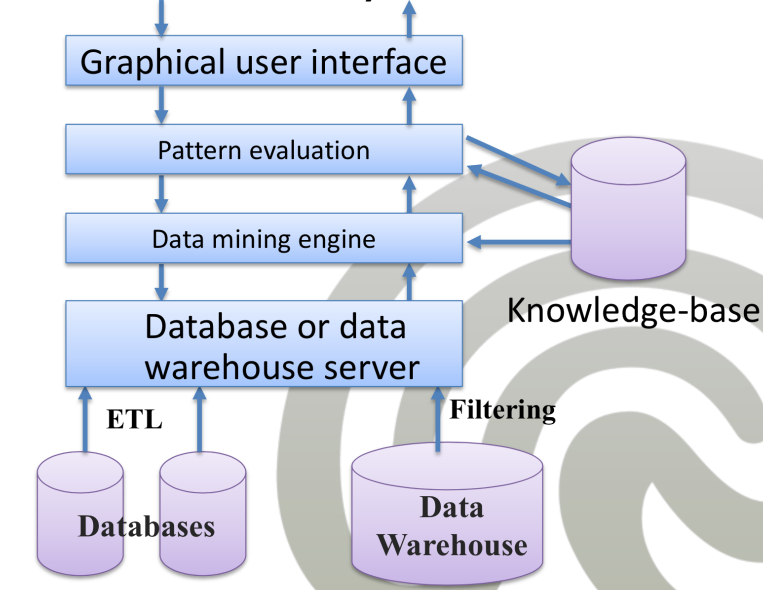
Data Mining Techniques
- Association (correlation and causality, find rules)
- Classification + Prediction (find models, decision-tree, classification rule)
- Cluster analysis (class label unknown, group data)
- Outlier analysis (Noise or exception)
Association Rule Mining
General
- Objective: Find co-occurrence relationships in data items
- Classical application: Market basket analysis
- Basic concept:
- Items \( I=\{i_1,...,i_m\} \)
- Transactions \( T=\{t_1,...,t_n \mid t_i\subseteq I\} \)
- AR: \( X\rightarrow Y, X \subset I, Y \subset I, X \cap Y = \emptyset \)
- Finding Association rules:
- Different strategies, result always the same
- Apriori algorithm
- Multiple minimum supports
- Mining class association rules
Quality
- Support \( X\rightarrow Y \):
- Percentage of transactions with items of rule and total transactions
- \( conf(X\rightarrow Y) = P(X,Y \in t_i) \)
- Low support -> Rule rarely useable
- Confidence \( X\rightarrow Y \):
- Percentage of transactions with X and Y and transactions with X
- \( conf(X\rightarrow Y) = P(Y \in t_i \mid X \in t_i) \)
- Low confidence -> Rule not reliable
- Objective
- Find all rules with support and confidence greater than threshold
Apriori Algorithm
- Step 1: Generate frequent item sets
- Step 2: Generate rules
- Frequent itemset
- Itemset with minimal support
- Apriori property / downward closure property:
- Any subset of a frequent itemset is a frequent itemset
- Optimization: Sort items in lexicographic order
- At most k (size of largest itemset) passes over data
- Problem: Data not equally distributed, impossible to find rules for rare items (through threshold)
Step 1: Find frequent itemsets
- Steps
- Initial step (find itemsets with size 1)
- Generalization of candidates (Find possible frequent itemsets, choose actually frequent itemsets)
- Generalization of candidates
- Input: \( F_{k-1} \)
- Output: Candidates
- Join step
- Generate possible candidates itemsets
- Candidate is only one element bigger than \( F_{k-1} \)
- Prune step
- Remove candidates violating the downward closure property
- Watch all subsets (compare to input set)
- Join step
Step 2: Generate rules
- Split each frequent itemset I into two disjoint proper subsets X and Y
- Test each two subsets:
- Confidence >= minconf
- Support(X->Y) = Support(I)
- Confidence(X->Y) = support(I) / support(X)
- Necessary information: support(I) and support(X)
- Information already obtained during generation
- Dont read transaction again
- Less time-consuming than generation of FI
Multiple minimum supports
- Rare item problem (Frequencies of items vary significantly)
- If minsup too high, rare-item-rules are not found
- If minsup low, combinatorial explosion
- Idea: Each item has minimum item support
- Problem: Frequent and rare items appearing in same itemset
- Solution: Support different constraint PHI
- Supports should be in equal magnitude
- Minsup of a rule
- Each item has user-specific minimum item support (MIS)
- \( support(R) >= min(MIS(i_1), ..., MIS(i_n)) \)
- Advantages:
- More realistic model
- Find rare items without huge number of nonsense
- \( MIS=100 \% \): Ignore item
Algorithm
- Extension of Apriori-Algorithm
- Problem: Downward closure property invalid (new item could lower minsup)
- Solution: Sort all items by MIS
- Steps
- Frequent itemset generation
- Initial step (Generate seeds)
- Candidate generation (k=2)
- Generalization (k>2)
- Join step
- Prune step
- Generation of rules
- Frequent itemset generation
Step 1.1
- Goal: Generate seeds
- Input: Items I
- Output: Seeds L, F1
- Steps
- Sort Items by MIS
- Calculate support
- Find first item x with sup(x) > MIS(x) and put in L
- For each item y (after x) with sup(y) > MIS(x) put in L
- Calculate F1 from L
Step 1.2
- Candidate generation
- Important: Use L, not F1 (Downward closure invalid)
- Input: Seeds L
- Output: F2
- Steps
- Take each seed x and check sup(x) >= MIS(x)
- If true, form 2-level-candidate with x and every other seed
- If false, continue
- Check candidates {x,y}: (sup(y) >= MIS(x) and |sup(x) - sup(y)| <= PHI
- Pass data again
- Validate candidate condition sup(x, y) >= min(MIS(x), MIS(y))
- Take each seed x and check sup(x) >= MIS(x)
Step 1.3
- Generatization
- Input: L_k-1
- Output: Candidates of all frequent k-itemsets
- Join step:
- Take two k-1 itemsets
- Join them with one different item (sort) -> I_k
- Respect support difference constraint
- Prune step:
- Remove (k-1)-subset S which is not in Fk-1
- Exception
- S does not contain first item of I_k
- If S(0) > I_k(0), keep. Else delete
Step 2
- Rule generation
- Head-item probem
- Confidence(A,B -> C) = sup(A, B, C)/sup(A,B)
- Read data again
Class Association Rules
- Define rules with targets
- Tools:
- Weka + RapidMiner
Sequence Patterns
Sequence patterns
- Goal: Mine ordered events, no concrete notion of time
- Applications: Customer retention, targeted marketing, Market prediction
- Event: Unordered list of items \( (I_2, I_1,I_3) \)
- Sequence S: Ordered list of events \( \langle e_1 e_2 e_3 \rangle \)
- Length of sequence: Number of items in sequence
- Sequence with length k: k-sequence
- Subsequence/supersequence: Ordering is kept
- Sequence database: \( S = \langle SID, s \rangle \)
- Support of sequence: \( sup_s(\alpha) = |\{ \langle SUP, s \rangle \mid ( \langle SUP, s \rangle \in S \land \alpha \in s)\}| \)
- Frequent sequence/sequence pattern/k-pattern: Sequence s with \( sup(s) >= minsup \)
Challenges + Mining
- Challenges:
- Huge number of possible sequential patterns
- Mining algorithm
- Find complete set of patterns
- Highly efficient
- Scalable
- Only small number DB scans
- Respect user-specific constraints
- Algorithms
- Apriori-based: Generalized sequential patterns (GSP)
- Pattern-growth methods: FreeSpan & PrefixSpan
- Vertical format-based mining: SPADE
- Mining closed sequential patterns: CloSpan
Generalized Sequence Patterns
- Downward closure: Sequence s is infrequent. Then none of its superclasses are frequent
- Steps
- Initial step: Collect items
- General step
- Scan database for support of candidates
- Remove candidates violating minsup (because downward closure)
- Generate length 2 candidates (2 event and 1 event)
- Drawbacks:
- Huge set of sequences
- Multiple scans needed
- Inefficient for mining long patterns (exponential)
Time-Series Data
- Sequence pattern with time (recorded intervals)
- Reveal temporal behavior
- Applications
- Financial
- Industry
- Meteorological
- Goals of analysis:
- Modeling
- Forecasting (Predict future values)
- Methods:
- Trend analysis
- Similarity search
Trend analysis
- Application of statistical techniques (regression analysis)
- Create model to explain behavior
- Characteristic time-series movements (components)
- Trend (T): Long-term procession
- Seasonal (S): Seasonal fluctuations, Similar movement during corresponding months
- Cycle (C): Regular fluctuations
- Irregular (I): Random, irregular influences
- Decomposition
- Additive model: Time series = T+C+S+I
- Multiplicative model: TIme series = TCS*I
Regression analysis
- Popular tool (find trends, find outliers, analyze time series)
- Dependent variable on independent variable
- Linear regression model most simple
- Non-linear regression or Bayesian
- Linear regression model
- Y = b0 + b1X1 + bnXn (bi: Unit of change)
- Correlation R: Interdependence of variable
- Regression trend channels (RTC)
- Standard deviation of linear regression (Trend line)
- Three parallel lines: Center line (regression), Upper and lower line (standard deviation)
- Problem: Can’t capture all real-world application
- Solution: Decompose time-series into basic movements
Basic movements T
- Trend analysis methods:
- Freehand (costly, unreliable)
- Least-square
- Moving-average
- Moving average
- Eliminates C,S,I patterns
- Loss of end data
- Flattens curve
- Sensitive to outliers
- Weighted moving average (handle outliers)
- WMA(3) with (a, b, c) = (ax + by + cz) / (a+b+c)
- Cumulative moving average (CA)
- Exponential weighted moving average (EWMA)
Basic movements S
- Seasonal variations (S)
- Seasonal index
- Show relative values of variable during months
- e.g. Ratio of monthly data and average of year
- Deseasonalized data
- Data adjusted for seasonal variations
- Divide/subtract original data by seasonal index
- Seasonal index
Basic movements (C + I) + Forecasting
- Cyclic variations (C)
- Same index as seasonal index
- Irregular variations (I)
- Adjust data for trend, seasonal, cyclic variations
- -> Long- or short-term predictions (time-series forecasting)
- Forecasting:
- Find formula that generates historical patterns
- Popular model: Auto-regressive integrated moving average (ARIMA)
Similarity search
- Goal: Find slightly differing data (DB only exact)
- Problem: Identify similar time series
- What is similarity?
- Symmetry in analogy or resemblance
- Similarity measure: Distance function
- Applications:
- Financial market (stocks, similar trend)
- Market basket (products, similar sales)
- Scientific databases (similar voice-clips)
- Categories of queries:
- Whole matching (find sequences which are similar)
- Subsequence matching (find sequences with similar subsequences)
Issues
- Issues:
- False alarms (False positive)
- False dismissals (False negative)
- Goal
- Correctness (avoid false dismissals)
- Efficiency (avoid false alarms)
- Reduction
- Problem: Large size/high-dimensionality (slow)
- Discrete Fourier transform (DFT)
- Concentration of energy (first few coefficients -> large waves (basic behavior))
Whole matching
- Idea
- Use euclidian distance
- Use multi-dimensional index (R-Tree) for DFT coefficients
- Use dimensionality-reduction (DFT, Wavelet)
- Guarantees no false dismissals (Parseval’s Theorem)
- Parseval’s theorem:
- Distance between two distance in time domain is same as distance in frequency domain
- Method:
- Index building
- Compute first k DFT coefficients
- Build index (2k dimensions, k complex)
- Query processing
- Compute DFT query sequence
- Use index -> find MBR for similar query (EPSILON)
- Compute actual distance (no false alarms)
- Index building
Subsequence matching
- Idea
- Extract sliding windows from sequence (whole matching of subsequences)
- Fourier transform each window (-> points)
- Trail: Function in Fourier space (moving windows)
- Index trails with MBR (R-Tree)
- Approaches
- Sliding window (expensive, but precise)
- Window matching (cheap, but more loss of information)
Method
- Index building
- Extract sliding window per sequence in DB
- Fourier transform windows to get trails
- Divide trails into sub trails for indexing
- Build R-Tree
- Query processing
- Extract p disjoint windows from query
- Fourier transform windows
- For each window, filter sliding windows that are EPSILON/ROOT(P) away
- Compute actual distance between candidate and query (discard false alarm)
Transformation
- Problem: Time-series can have different scaling/baselines
- Solution: Use different transformations
- Shifting
- Scaling
- Normalization
- Moving average
- Dynamic time warping
Enhanced methods
- Enhanced methods
- Allow gaps in sequence
- Normalize amplitude and offset
- Envelopes (width EPSILON)
- Non-overlapping, time-ordered pairs
- Parameters (window size)
- Enhanced subsequence matching
- Index building
- Query processing
- Atomic matching
- Window stitching
- Subsequence ordering
- Enhanced whole matching
- Normalize one sequence (offset and scaling)
- Query languages for time-series
- Specify sophisticated queries
- Support range queries
Classification
General
- Goal: Find model (label as function)
- Training set (features, label)
- Test set: Validation
- Learning (Induction), Classification (deduction)
- Type of supervised learning (Labels known)
- Techniques/methods:
- Decision-tree
- Rule-based
- Naive Bayes
- Support Vector Machine
- Neural Networks
Decision trees
- Flow-chart-tree-structure
- Inner node: Attribute test
- Leaf: Class label
- Induction:
- Hunts algorithm (earliest)
- Different implementations of Hunts (ID3, C4.5, CART)
- Advantages:
- Inexpensive
- Fast
- Easy to interpret
- Accuracy comparable for simple data sets
- Good average performance
Hunt’s algorithm
- Node
- If record set from same class, node is leaf
- If not, node has an attribute test to split data set
- Greedy strategy
- Split records by attribute test to optimize criterion
- Issues
- How to split? (Attribute test condition, Quality of split)
- When to stop splitting?
Attribute testing
- Splitting
- Depends on attribute type (nominal, ordinal, continuous)
- Depends on number of ways (binary, n-ary)
- Continuous attributes
- Discretization (ordinal category
- Static (discretize on beginning)
- Dynamic (equal interval bucketing, clustering)
- Discretization (ordinal category
- Determine best split
- Prefer nodes with homogenous classes (pure nodes)
- Measure with information gain
Information gain
- Assumption (C4.5): All attributes categorical
- Method:
- Classes P and N
- Information needed to decide whether element is in P or in N
- Select attribute with highest information gain
- \( I(p,n) = -\frac{p}{p+n} \log_2 \frac{p}{p+n}-\frac{n}{p+n} \log_2 \frac{n}{p+n} \)
- Entropy
- Expected information needed to classify
- \( E(A)=\sum_{i=1}^v \frac{p_i+n_i}{p+n} I(p_i, n_i) \)
- \( Gain(A) = I(p,n)-E(A) \)
- Divide until stop
Stop condition
- Option 1: All records belong to same class
- Option 2: All records similar attribute values (majority class label)
Deduction + Classification rules
- Use decision rules
- Classification rules
- Extract rule from tree
- IF-THEN-Form
- One rule per path
- Conditions form conjunction
- Leaf node: Class
- Advantage: Easy to understand
Overfitting
- Result: Too many branches, poor accuracy for unknown elements
- Prepruning
- Halt construction early (Information gain threshold, difficult)
- Postpruning
- Iteratively remove branches (test trees with test set)
- Bucketing of continuous-valued attributes
- Missing attribute values
- Assign common value or probability
- Attribute construction (merge sparsely represented attributes)
Bayesian Classification
- Probabilistic learning
- Incremental (each sample changes probability)
- Assumption: Statistical independence
- Bayes’ Theorem
- \( P(A|B) = \frac{P(A)}{P(B)} * P(B|A) \)
- Probabilities obtained from training data
- Classify new: Compare \( P(p|X) \) and \( P(n|X) \)
- Summary
- Robust to noise
- Robust irrelevant
- Independence unrealistic
SVM
- main classification tool
- Assumptions
- Binary classification
- Vector representation
- Task: Find linear classifier (divide R^n)
- Quality of separator
- Idea: Margin of line
Maximum margin classifier
- Classifier with maximum margin
- Linear SVM
- Assumption: Training set linearly separable
- Why maximum margin?
- Intuitive
- Best against errors
- Robust
- Empirically good
- Soft margins (Handle noise)
- Mistakes allowed
- Misclassification gets error value
- Minimize total classification error
- More classes?
- One-versus-all (one SVM per class)
- One-versus-one (one SVM per class-pair)
- Multi-class SVM
Overfitting
- Too much dimensions -> overfitting
- Cross-validation:
- Randomly split data
- Choose SVM which maximizes performance
- Regularization:
- Penalty for an expected classifier (e.g. polynomial)
- Optimize original goal + penalty
- Example: Soft margin technique
Clustering
General
- Unsupervised learning (class label unknown)
- Cluster Analysis
- Goal: Find structure in unlabeled data
- Def.: Organize objects into groups with similar members
- Applications
- Market research
- Pattern recognition
- Data analysis
- Information retrieval
- Image processing
Requirements
- Scalability (large data sets)
- Deal with different types of attributes (binary, categorical, ordinal data)
- Discover clusters of arbitrary shape (usually sphere)
- Deal with noisy data
- High dimensionality
- Minimal requirements of domain knowledge (parameters difficult)
Issues
- How many clusters?
- Number of clusters k (defined, undefined)
- Flat/hierarchical
- Flat: All clusters at once, iteratively reallocate items
- Hierarchical
- Agglomerative (merge items to larger clusters)
- Divisive (split clusters)
- Hard/soft
- Hard: Every item exactly one cluster
- Soft: Multiple clusters
Problem + Goals
- Task: Find clustering minimizing cost function
- Given: Collection of items, type of clustering, cost function (usually distance)
- Internal/structural criteria
- Primary goals:
- Low inter-cluster similarity
- High intra-cluster similarity
- Secondary goals:
- Avoid very small clusters
- Avoid very large clusters
- External criteria
- Compare clustering against hand-crafted reference clustering
- Primary goals:
- Naive: Try all clustering (count: S(n, k) hard, flat clusters)
Flat clustering
- K-means (represented by center)
- K-medoids (represented by object)
- PAM (Parition around medoids)
K-means
- Important hard, flat clustering
- Defined \( k \)
- Data points unit vectors
- Objective: Minimize avg. distance from object to center
- Center/centroid: \( \mu (A) = \frac{1}{m} \sum_{i=1}^m d_i \)
- Quality of cluster: Residual sum of squares (RSS): \( RSS(A)=\sum_{i=1}^m ||d_i - \mu (A)||^2 \)
- Quality of clustering: \( RSS(A_1,...,A_k) = \sum_{i=1}^k RSS(A_i) \)
- Goal:
- Minimize \( RSS(A_1,...,A_k) \)
- Minimize average squared distance between object and centroid
- Advantage
- Efficient \( O(nkt), t << n \)
- Often terminates local optimum
- Disadvantage
- Only if mean defined
- Need to define k
- Unable for noisy data/outliers
- No non-convex clusters
Lloid’s algorithm
- Lloid’s algorithm
- Create k empty clusters
- Assign random seed to clusters
- For each object: Assign to cluster with nearest centroid
- Recompute cluster centroids
- Recompute RSS
- If good enough, return to (3)
- Stop criteria:
- Small change per iteration
- Maximum number iterations
- Threshold for RSS
- Similar approaches
- K-medoids
- Fuzzy c-means (soft)
- Model-based (maximum likelihood)
Hierarchical clustering
- Set of nested clusters
- Visualize with dendrogram
- Agglomerative (bottom-up)
- Start with items
- Merge closest points
- Divisive (top-down)
- Start with one cluster
- Split clusters
Inter-cluster similarity
- Single-link similarity (MIN)
- Similarity of most similar neighbors
- Problem: Produces long chains of clusters
- Complete-linkage similarity (MAX)
- Most dissimilar members
- Problem: Sensitive to outliers
- Group average clustering
- Average of all similarities
- Problem: Computationally expensive
- Centroid clustering
- Average similarity in cluster
- Similarity between two clusters
- Problem: Similarity improves by merging
Agglomerative Clustering
- Algorithm
- Create cluster for each data point
- Compute similarity (mxm similarity matrix)
- Merge two clusters with maximal similarity
- If more than one clusters exist return to (2)
- Key operation: Similarity measure
- Inter-cluster similarity
- Single-link clustering (MIN)
- Complete-link clustering (MAX)
- Group average
- Distance between centroids
Divisive Clustering
- Idea: Iteratively clustering (e.g. 2-means)
- Constraints on quality:
- Avoid very small clusters
- Avoid splitting into clusters of extremely different cardinalities
Outlier Analysis
- Don’t comply general behavior
- Sources (correct data, bad data)
- Knowledge categories
- Incorrect
- Useless (obvious)
- New, surprising, interesting
- Outlier detection
- Problem: Multiple dimensions, not easy by visualizing
- Outliers don’t lie in cluster
- Outliers don’t behave like norm
- Methods
- Statistical
- Distance-based
- Deviation-based
Approaches
- Statistical
- Assume model (e.g. normal distribution)
- Problem: Most tests for one attribute, data distribution unknown
- Distance-based
- Goal: Multi-dimensional analysis without knowing distribution
- Object is outlier if not enough neighbors (by distance}
- Deviation-based
- Object deviation from description of groups
- OLAP data cube technique
- Cell is outlier if it differs from aggregate
- Compute expected value (regression)
- 3-Sigma-rule
Clustering in Data Warehouses
- Challenges
- High-dimensional data (many irrelevant dimensions, e.g. gender)
- Clusters may exist only in subspaces
- Large data set
- Handle high-dimensional data
- Feature transformation
- Concentrate energy (uses all dimensions, useful when clusters exist in high-dim space)
- Singular Value Decomposition, highly correlated/redundant attributes)
- Subspace-clustering (find clusters in subspaces)
- Feature transformation
CLIQUE
- Clustering in QUEST (first DW)
- Automatically find subspaces in high-dimensional data for better clustering
- CLIQUE density- and grid-based
- Dense unit: Total data points in unit exceed threshold
- Cluster: Maximal set of connected dense units
- Connected unit: Adjacent or diagonal
- Apriori principle in CLIQUE
- If k-dimensional unit is dense -> projection in (k-1)-dimensional also dense
- -> If (k-1) dimensional unit not dense -> prune k-dimensional unit
- Strength
- Find subspaces highest dimensionality with high density clusters
- Insensitive to order of records
- Linear scaling with input data
- Weaknesses
- Clustering accuracy may be degraded because of simplicity
Algorithm
- Identify subspaces with clusters
- Find dense units
- Level by level (start with 1)
- Generate k-dim. Candidates from k-1 dense units
- Check each candidate if its dense
- Find dense units
- Identify clusters
- Input: Set of dense units
- Output: Find partitions of connected units (U1…Uq)
- Depth-first search
- Generate minimal description for clusters
- Input: Partitions
- Problem: Cover units with minimum number of regions (NP-hard)
- Solution: Greedy algorithm
Minimum coverage
- Start with U1 and random seed
- From seed grow rectangle covering only units of U1
- Start with not covered units from U1 (1)
- Repeat for every cluster
Meta Algorithms
General
- Upper family algorithms -> For strategy
- Not problem-specific
- Use meta-heuristics / domain specific knowledge
- Last resort (don’t know how to find solution)
- Prerequisite: Ability to grade result
- Application: Multi-classifier combination
- Single classifier poor accuracy
- Together: Strengthen each other
Genetic algorithms
- Mimic nature (selection, recombination, mutation)
- Mutation: Evolve solution to problem
- Components
- Encoding: genes/chromosomes
- Initialization: creation
- Evaluation: Environment
- Selection of parents: reproduction
- Genetic operations: mutation/recombination
- Evaluation: Fitness score (how good chromosome evolves)
- Selection: Proportional to fitness score
- Recombination: Crossover of two chromosomes
- Mutation: Flip bits dependent on mutation rate (0,001)
- Repeat until population of N reached, stop if one chromosome solves
Genetic algorithms structure
Initialize population
Evaluate population
  While TerminationCriterionNotSatisfied {
  	 	Select parents
  		Perform recombination/mutation
  	 	Evaluate population
   }
Bootstrapping
- vim + assembler -> Java
- Seed AI
- AI improving itself
- No such system exists
- Bootstrap:
- Idea: Sampling with replacement
- Build sample (length N) by sample with replacement from sample
- Repeat 1000 times -> Distribution of averages (variance)
- High variance -> good (more diversity, less bias of base set)
Bagging
- Bootstrap aggregating
- Build new training set (sample with replacement)
- Train classifier on sample
- Repeat m times -> m classifiers
- Classifying:
- Perform majority vote
- Advantage
- Increases stability
- Reduces variance (small changes for unusual objects)
Boosting
- Based on bagging
- Idea
- Build series of classifiers (on single training set)
- Pay attention to misclassified examples of predecessor
- Concept
- Blueprint of combining classifiers to better classifier
- Each classifier own stengths/weaknesses
- Hard problem -> Weak learners
- Set of weak learners -> Strong learners
- Naive approach: Majority vote
- Train base classifiers on training sets
- Classification: Ask each classifier -> majority vote
- Problem
- Works only if majority is right often
- Expert vote as same as other vote?
Adaptive boosting
- Steps
- Train base classifier
- Check mistakes (errors)
- Assign weight (low = correctly, high = mistake)
- Train new base classifier on weighted set
- Reweight as in (3)
- Repeat (4) and (5)
- Finally: Importance weight (believability)
- Hight importance: Few errors on high-weighted objects
- Low importance: Lot errors on high-weighted objects
- -> Should be balanced
- Why better than pure majority vote?
- Compensate individual weaknesses
- Exploit individual strengths
Formalization
- Instance space \( X \)
- Class labels \( Y \)
- Training set \( \{\{x_i,y_i\}\} \)
- Iterations \( T \)
- Vector \( D_t \) per training item with weights for each iteration
- \( D_i = 1/m, 1< i< m \)
- Generate weak learner: \( h_t:X\rightarrow Y \)
- \( h_t = \arg\max |0.5-e_t| \) with \( e_t = \sum_{i=1}^m D_t(i)*I_{y_i \neq h_t(x_i)} \)
- High error on boosted item -> high error rate
- Test \( h_t \) on training examples
- Find suitable value for \( T \)
- Stop condition: \( |0.5 - e| < b \) (quality threshold)
Deep Learning
Biological Learning
- Neutrons propagate electro-chemical signals
- Connection: Synapse
- Signal triggers cell (signal greater threshold)
- Artificial learning
- Goal: Computational model (mimic brain learning)
- Approach: Different algorithms per task
- Idea: One algorithm
Applications of learning
- Image colorization
- Object classification/detection
History of deep learning
- Started in 1940
- Norbert Wiener: Control/regulation mechanisms in humans
- Waves of development
- Cybernetics (1940-1960) (Perceptron)
- Connectionism/neural network (1980-1990) (Back propagation, hidden layers)
- Deep learning (2006-)
Artificial Neural Networks
- Model brains biological structure
- Organized in layers (Interconnected neurons, activation function)
- Activation function: Compute output from input
- e.g. threshold, linear, sigmoidal
- Input layer
- Hidden layer
- Output layer: Meaningful transformation of input
Perceptron
- Smallest unit
- Receives n input
- Signals transmitted over weighted synapse
- Sum input singles up
- Weights
- Set using a-priori domain knowledge
- Deduce by re-weighting (supervised, unsupervised)
Architectures
- Feed-forward neural network: Information only one direction
- Recurrent neural network
- Feedback information
- Remember information
Feed-forward
- May have zero/multiple hidden layers
- No feedback connections
- Types
- Single-layer perceptrons
- Multi-layer perceptrons
- Issues
- Not linearly separable (no convergence)
- No maximum margin (no improvement if solution found)
Perceptron algorithm
- Input layer directly to output layer
- Supervised machine learning
- Modify weights: \( S=\sum_{i=1}^n w_i x_i \)
- Steps
- Initialize weights and threshold
- Input training patterns and compute output
- Update weights
- Back to (2) until max iterations or no weight change
- Optimal weights/performance of network
Multi-layer perceptron
- One/more hidden layer
- Non-linear functions
- Hidden layer
- Extract higher-level features
- Neuron detects specific output (weighted input/activation function)
Back propagation
- Problem: Direct feedback impossible (output needed)
- Delta learning algorithm
- Propagate deltas backward from output to input/hidden layers
- Goal: Adjust errors
- Gradient descent: Change weights in direction of biggest gradient
- Problems
- Slow (weight adjustment)
- Many poor local optimum
- Requires lot of training data
Algorithm
- Initialize weights
- Feed network with input
- For every input compare output of network with expected output
- Propagate delta back (delta=difference) to prev. layer
- Each layer re-computes new weights
- Repeat 4+5
- Update all weights
Deep Learning
- Amount available data increased
- HW/SW support improved
- Learning types
- Shallow learning (depends on prior knowledge, pure statistics)
- Deep learning (Extract complex representation)
- Architectures
- Recurrent Neural Net
- Convolutional Deep Neural Net
- Embedding
- Deep Autoencoders
- etc.
Convolutional deep net
- Inspired by animals visual system
- Idea: Learn complex representation of images
- Application: Speech/object recognition
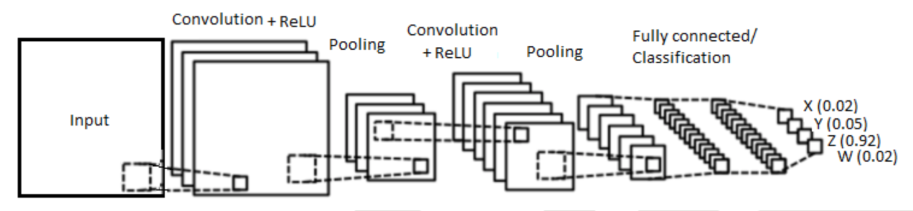
LeNet
- Convolutional Deep Netwerk
- Idea: Character recognition with probabilities
- Key operations
- Convolution
- Non-linearity
- Pooling/subsampling
- Classification
- Input
- Image as matrix of pixels (RGB, three matrices)
- Classification
- Fully connected layer
- MLP
Training
- Training
- Initialize kernels and weights
- Feed network with images
- Compute total error
- Back propagation
- Repeat 2-5
- Training phase output: ConvNet with optimized weights/kernel parameters
- Predict output: Label with highest probability
Convolution + Kernels
- Convolution
- Filtering to modify spatial frequency
- Filter out unnecessary information
- Multiply image with Kernel
- Result: Convolved image
- Kernel (filter/feature detector)
- Different kernels -> different features (edges, curves)
- The more kernels the more features
Rectified Linear Unit
- Filtering idea
- Apply after convolution (linear convolution)
- Get non-linearity
- e.g. remove negative
Pooling
- Dimensionality-reduction
- e.g. max-pooling, avg-pooling
- Retain relevant dimensions
TensorFlow
- Open source deep learning framework
- Developed by Google
- Tensor: Multidimensional array structure
- Tensors flow through data graph
- Nodes: Opersations (receive/output tensors)
- Learning rate: How fast to adjust weights