Data Warehousing
General
What is a data warehouse?
- Large database
- starts at one TB
- Several servers
- Impressive amount of computing power
- collective data repository
- Snapshots operational data
- Purpose: Analytics
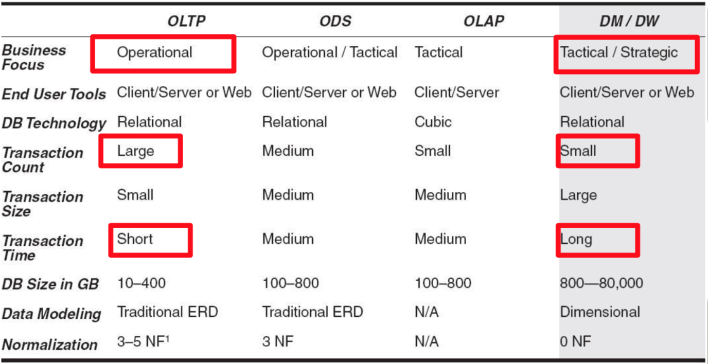
- Tactical/strategic focus
- Implies small number transactions
- Large transactions (long running)
Comparison OLTP/ODS/OLAP/DW
Definition
- Kimball: Copy transaction data, specifically structured, query and analysis
- Inmon: Subject-oriented, integrated, non-volatile, time-variant collection of data in support of managements decisions
- General: Large repository of organizations data, specifically designed for reporting and analysis
Inmon-Definition
- Subject-oriented: Relate same real-world/linked together
- Integrated: data from most/all ODS and is consistent
- Non-volatile: Data never over-written or deleted, real-only; data is loaded, not updated
- Time-varying: Change over time; time horizon: 19 years
DW Features
- Run on enterprise scale DBMS (Oracle, Teradata)
- Retain data long periods of time
- Consolidate data from various sources
- Have own carefully designed data model
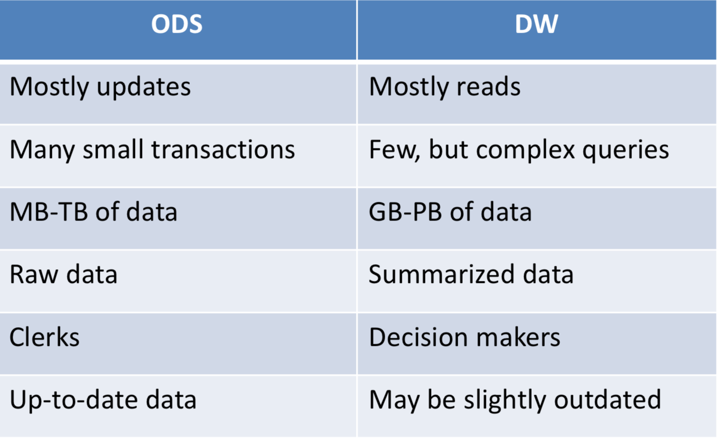
OLTP vs OLAP
- OLTP:
- Typically for data entry / retrieval
- Works on operational data store
- Only current state
- OLAP:
- front-end analytics
- Reporting / decision oriented
Application of DWs
- front-end analytics
- Result: Data visualization, reporting
- OLAP: Provide timely (relative term), accurate, understandable information
- KDD: Constructs models of data
Users of DWs
- Decision support system analysts
- Define / discover information used for decision-making
- Explorative line of work
- Defines how the DW is developed
DW Lifecycle
- CLDS: Implementation, Integration, Test, Program, Design DDS, Analyze results, understand requirements
- Data-driven development
- Design: Interview end-users, analyze ODS, define key performance indicators, map decision-making processing, logical/physical schema
- Prototype: Costrain and reframe end-users requirements
- Deployment: Documentation; personal training
- Operation: Day-to-day-maintenance, ETL
- Enhancement: HW/physical components; logical schema design
Operating a DW
- Monitoring
- Extraction
- Transform
- Load
- Analyzing
Monitoring phase
- surveillance operational data source
- Identification of data modification relevant
- Techniques
- Active mechanism (Event condition action)
- Replication mechanisms
- Protocol based mechanisms (Logging)
- Application managed mechanisms (time stamping, data comparison)
Extraction phase
- read selected data and insert into staging area
- depends on hardware
- Time-point of extraction
- Periodical
- On request
- Event driven
- Immediate
Transforming phase
- implies adapting data, schema and data quality to requirements
- Data Integration: denormalization, key attributes, different data types, conversion, encoding, strings, measurements units, aggregation
- Data cleansing: consistency check, completeness, regex, duplicate detection, redundancy elimination
Loading phase
- load when system is not under stress
- initial load / periodical load
- Initial load: big data volumes; bulk loading
Analyzing phase
- data access (extract data for business goals)
- OLAP
- Data mining
Architecture
Architecture
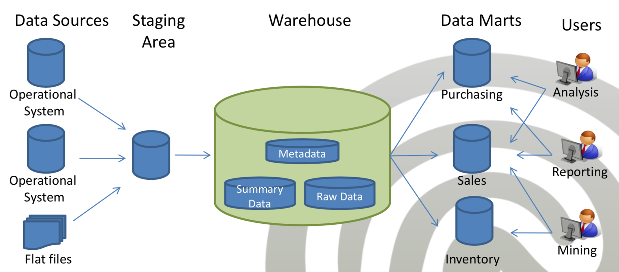
Operational Data Store
- Database for daily operations
- Normal RDBMS
- Small queries
Staging Area
- Separate copy of data loaded from ODS to DW
- Preparation for DW
- For DW professionals only
Data Warehouse
- Content
- cleaned raw data
- Derived / aggregated data
- Metadata (meaning, properties, origins)
- Build a DW
- Hardware and data flow architecture (ETL)
- Storage structure
- Data modeling (conceputial, logical, phyiscal)
Presentation Area
- „Data Warehouse“ for the business community
- Data Mart for one department
- Data Mart usually DB materialized view
- Analytical processing
Architectures in practice
- Vertical tiers
- Generic two-tier
- Three-tier
- N-tier (possible, complexity grows)
- Web-based architectures (usage existing software, cost reduction, platform independent, security overhead, data encryption)
- Horizontal tiers
- Independent data mart
- Dependent data mart
- Logical data mart
Two-tier
- Generic client-server architecture
- Thin client
- operations executed on server
- Client usually displays results
- Internet DW access
- Fat client
- server selivers data (data mart)
- Operations executed on client
- Large data transfer
Three-tier
- Tier 1: Raw + detailed data single source for DSS
- Tier 2: Derived data
- Tier 3: Reporting analysis
Independent data mart
- Mini warehouse / limited in scope
- Faster and cheaper
- Redundant processing
- Separate ETL for each Data Mart
Dependent data mart
- Single ETL
- No redundancy
- Data Marts are loaded from the DW
Logical data mart
- Data Mart are not separate databases
- Data Mart logical view
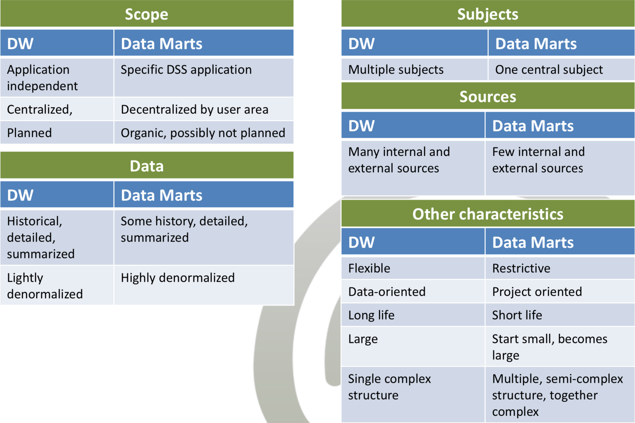
DW vs. Data mart
Centralized and distributed DWs
- Centralized DW
- Analytical queries only at main enterprise location
- Hight costs for large dedicated hardware
- No networking
- Distributed DW
- „Natural form“ Company active all over the world
- Higher overhead
- Lower cost
- Types:
- Geographically distributed
- Technologically distributed
- Independently evolving distributed
Geographically distributed DW
- Case: Corporate spread around the world
- Information needed locally and globally
Technologically distributed DW
- DW on distributed technology of some vendor (Amazon)
- Advantage: Low entry costs (large centralized hardware), no theoretical limit
Independently evolving distributed DW
- Development concurrently in same company
- Uncontrolled growth
Conceptual modeling
Relational / multidim. Model
- Storage either relational or multidimensional
- Advantage multidimensional
- Ease of data presentation
- MD: Presentation is natural output
- RM: Complex query
- Ease of maintenance
- MD: Maintain aggregates on insert
- RM: Index and storage maintenance
- Performance
- MD: Transformation is performed on load
- RM: For each query, transform from relational to multidimensional, tune to reach similar performance
Data modeling in DW
- Models must support multidimensional data
- Relational model goal: Remove redundancy, efficient retrieval for individual records
- DW goal: Redundancy is necessary to speed up queries, OLAP involves multiple records (range queries) and aggregates
Multidimensional conceptual model
- Model business queries
- Define the purpose of DW and subject
- Identify questions of interest (Who buys products? What is sold? When was it sold?)
- Components of conceptual design
- Facts: Focus of interest
- Measures: Attribute that describe facts from different points of view
- Dimensions: Discrete attribute which determine granularity for facts
- Hierarchies: Made up of dimensions (aggregation level)
- Design models
- Multidimensional Entity Relationship Model (ME/R)
- Multidimensional UML (mUML)
Multidimensional E/R
- Purpose: Create intuitive representation
- Multidimensional semantics
- ME/R was influenced by considerations
- Specialization of E/R model (Expressiveness of E/R is not reduced)
- Minimal expansion of E/R model (Additional elements should be small)
- Representation of multidimensional semantics (Should be powerful)
- ME/R constructs
- Fact node
- Level node (Basic classification level: smallest granularity)
- Classification edge
mUML
- UML general purpose modeling language
- Taylor to specific domains using stereotypes, tagged values and constraints
- Stereotypes (new elements)
- grants special semantic without modifying UML construct
- Tagged values (new properties)
- define properties by a pair of tag and data value
- Constraints (new semantics)
Logical modeling
Logical Model
- Elements: Dimensions and cubes
- Basic operations: Cube-selection, -projection, -join
- Change support for logical model
- Goal
- Refine real facts and dimensions in the conceptual model
- Establish granularity of dimensions
Dimensions
- Dimensions are entities (from data model for analysis)
- Hierarchically organized
- Organized in classification levels (called granularities)
- Dependencies described in classification schema by functional dependencies
- Functional dependency: A->B iff for every a exists exactly one b
- Comparing granularities
- Granularity \( G = \{D_1.K_1, ..., D_g.K_g\} \) is finer than \( H = \{D_1'.K_1',..., D_h'.K_h'\} \) iff for each \( D_j'.K_j' \) from \( H \) there is a \( D_i.K_i \) from \( G \) where \( D_i.K_i \rightarrow D_j'.K_j' \)
Classification schema
- Classification schema of a dimension D is semi-ordered set \( (\{K_1,...,K_k\}, \rightarrow) \) of classification levels
- Smallest element \( D.K_0 \) (no classification level with smaller granularity)
- Fully-ordered set of classification levels is a Path
Classification hierarchies
- Classification hierarchy concerning a specific classification schema
- Classification hierarchy is balanced tree
- Nodes from \( dom(K_1) \cup dom(K_k) \cup \{ALL\} \)
- Edges respect functional dependency
Cubes
- Basic unit of multidim. paradigm
- Store measures in raw and pre-aggregated form
- Definition from slide 3.12
- Aggregates sepeed up queries
- Representation as lattice of cuboids (0-D-apex-cuboid highest summarization and n-D-base-cuboid contains the non-non-aggregated values)
Basic operations
- Selection
- Projection
- Cube join
- Aggregation
MD Selection
- Definition from slide 3.17
- Selection over predicate P
- Variables in P can be classification levels K with \( D.K\rightarrow K \) or Measures
MD Projection
- Measure \( F(M) \)
- Definition from slide 3.18
MD Join
- Join is usual (calculate missing values from cube)
- Join only possible if granularities are equal
- Otherwise aggregate
MD Aggregation
- Join with unequal granularities requires aggregation
- Aggregation most important operation for OLAP
- Functions: SUM, AVG, Count
Support change of classification hierarchies
- Schema and hierarchy are fixed
- Reasons hierarchy can change: New requirements, data evolution
- Problem: One product only one category (Samsung O2XDA with GSM and 3G)
- Solution: Introduce versioning with validity timestamps
- Storage: Store as metadata as validity matrix (Rows parent nodes, columns child nodes)
Schema versioning
- No data loss
- All data corresponding to all schemas always available
- Old data is held in old schema
- Advantages
- High flexibility
- Disadvantages
- Adaption of data is done at runtime
- Longer query run time
Schema modification / evolution
- Just one schema
- Modification without data loss
- Involves data adaption to new schema
- Advantage: Faster queries
- Disadvantage: Limits user flexibility, only schema supported
Physical modeling
Physical model
- Define physical structures
- How to access data and how to arrange data
- Performance tuning strategies
- Indexing
- Partitioning
- Materialization
- Data in DW is stored according to multidimensional paradigm
- Existing physical models
- MOLAP
- ROLAP
- HOLAP
- DOLAP
Multidimensional model
- Basic data structure: Array
- Elementary data structure are the cubes and the dimensions
- Storage of matrices as arrays of arrays: Linearization
Linearization
- Index
- Problems
- Influence of the order of the dimensions
- Storage of dense cubes
- Storage of sparse cubes
Problems in linearization
- Influence of the order of the dimensions:
- After linearization information of columns is spread over blocks
- Solution: Caching (MDBMS own caching to prevent OS)
- Storage of dense cubes
- Storage efficient
- Large loading times
- Solution: Store dense cubes not linearly but on two levels
- First level contains indexes
- Second level contains data cells
- Optimization: Indexes, physical partitioning, compression
- Storage of sparse cubes
- Store empty cells
- Read speed slower
- Solution
- Do not store empty blocks/pages (adapt index structure)
- 2 level data structure: Upper layer hold possible combinations of sparse dimensions, lower layer holds dense dimensions
Multidimensional to relational
- Goals relational model
- Low loss of semantic knowledge
- Translation of multidimensional queries must be efficient
- RDBMS should run translated queries efficiently
- Maintenance should be easy and fast
- Multidimensional to relational
- Representation for cubes, dimensions, classification hierarchies and attributes
- Implementation of cubes without the classification hierarchies is easy (fact table)
- Schemas
- Snowflake
- Star
- Starflake
- Galaxies (More measures by different dimensions -> more fact tables)
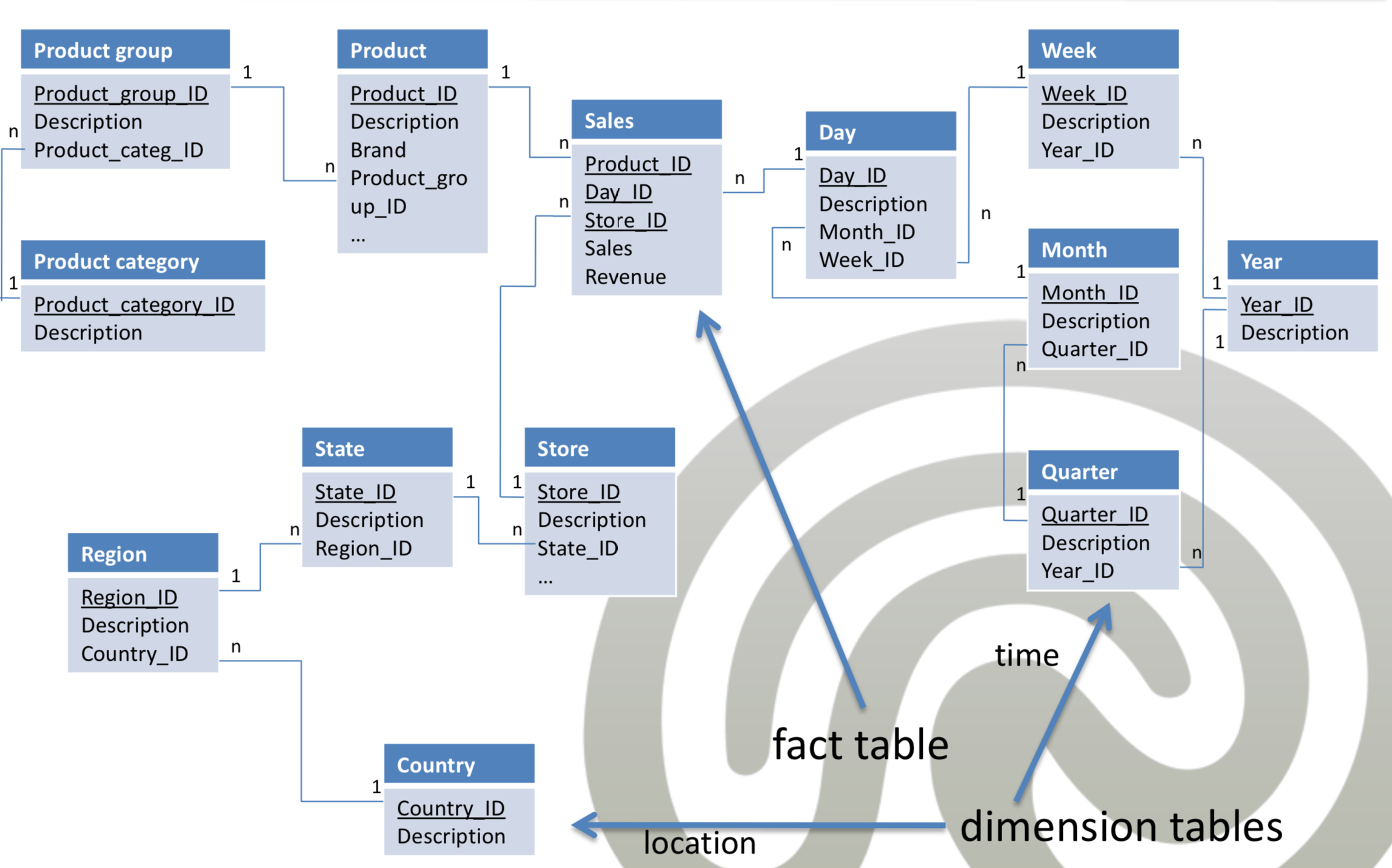
Snowflake-Schema
- Idea
- Tables for each classification level
- Measures in fact table
- Neighboring classification levels are connected by 1:n relationship
- Fact/measures in center
- Dimensions spread out in each direction and branch out with granularity
- Advantages
- Size of dimensions tables is reduced -> queries run faster
- Easier to maintain (no redundancy)
- More flexible querying with complex dimensions
- Disadvantages
- Normalizing reduces performance -> Large number of tables, join at query time
Star-Schema
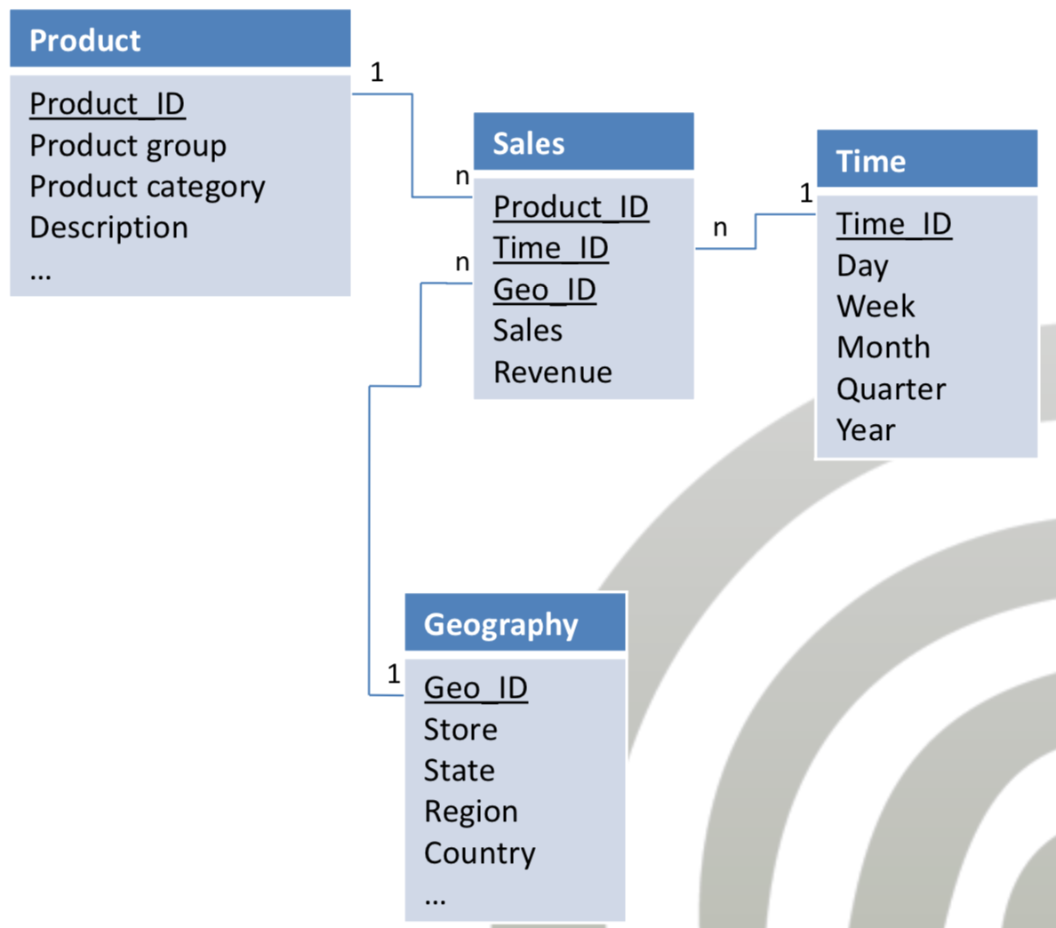
- Idea
- Use denormalized schema for all dimensions
- Can be obtained by denormalizing snowflake-schema
- Advantages
- Improves query performance (often used data)
- Less tables
- Simples structure
- Efficient query processing
- Disadvantages
- High overhead of redundant data
- No many-to-many-rels (one week, two months)
Snowflake- and star-schema
- Snowflake
- Structure of classifications are expressing table schema
- Fact and dimension tables are normalized
- Star
- Entire classification in one table
- Fact table normalized while dimension tables aren’t (redundancy)
- When to move from snowflake to star?
- Heuristics-based decision
- typical queries relate to coarser granularity (more joins)
- Volume of dimensions relatively low compared to fact table
- Modifications on classifications are relatively rare
- Heuristics-based decision
- Snowflake or star?
- depends on necessity (fast query processing or efficient space usage)
- Usually a mixed form is used: Starflake schema
Starflake-schema
- Which dimensions should be normalized?
- Frequency of modifications (dimensions that change often should be normalized)
- Amount of dimension elements (the bigger the dimensions the more space normalization saves)
- Number of classification levels in a dimension (more levels more mean more redundancy in star schema)
- Materialization of aggregates (if aggregation is materialized, normalization of dimension can bring better response time)
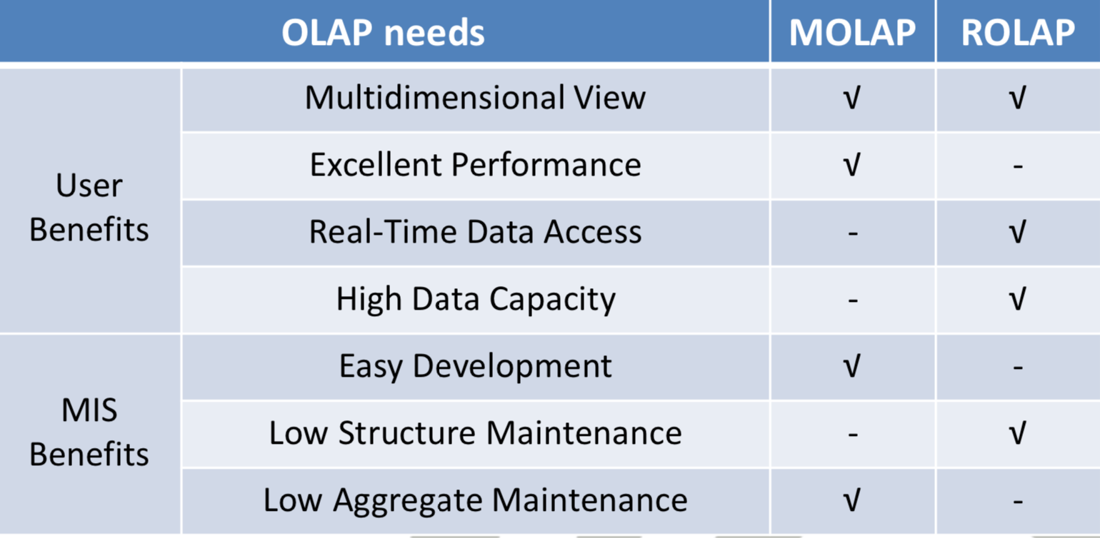
MOLAP
- Presentation layer provides multidimensional view
- Server stores data in multidimensional structure
- Pre-aggregations occurs during loading step
- Advantage: Excellent performance (all values generated when cube is created)
- Disadvantage
- Enormous overhead
- Limited amount of data can be handled
- Requires additional investment (Proprietary)
ROLAP
- Schema: Star or snowflake
- Special indexes: Bitmap, R-Tree
- Advantage: Proven technology (RDBMS), Can handle large amounts of data
- Disadvantage: Limited SQL functionality
MOLAP vs ROLAP
HOLAP
- Hybrid MOLAP and ROLAP
- Vertical partitioning
- Aggregations store in MOLAP (fast query performance)
- Details stored in ROLAP (optimize time for cube processing)
- Horizontal partitioning
- Store recent slice of data (time dimension) in MOLAP for fast queries
DOLAP
- Download small hypercube from central point
- Perform multidimensional analysis while disconnected from data sources
- Computation on client side
- Requires little investment
- Lacks the ability to large datasets
Indexing
Why indexes?
- Goal: Minimize size of read pages
- Problem: DW data is multidimensional, B-trees only one-dimensional
Tree structures
- Idea multidim. Trees
- Geometric regions describe a set of points
- Consider clusters only (not points)
- Hierarchical cluster
- Criteria
- Cluster construction: Local grouping/Completely fragmenting (uniform grid)
- Cluster overlap: Overlapping/disjoint
- Balance: Balanced/Balanced
- Object storage: In leaves and/or inner nodes
- Geometry: Hyper-sphere, hyper-cube
R-Trees
- Multidimensional extension of B-tree
- Used for low-dimensional applications (max. 10 dim.)
- Scalable versions: R+-, R*, X-Trees
- Dynamic index structure (CDU possible)
- Data structure:
- Data pages: Leaf nodes, store clustered point data and data objects
- Directory pages: Internal nodes, store directory entries
- Usage of Minimum bounding rectangles (MBRs)
Characteristics
- Local grouping
- Overlapping clusters (decrease in efficiency)
- Height-balanced tree structure
- Leafs: Objects
- Inner nodes: Navigation
- Geometry: MBR
- Properties
- Root at least two children
- Inner node: Between M/2 and M children
- All leaves: same level; between M/2 and M index records
- Inner node: MBR of children
- Leaf node: MBR of data
- Operations: Search, insert, update, delete, split
Search
- Recursive search from root to leaf
- Select one path (arbitrarily)
- If record not found, select next path
- No guarantee for good performance
- Worst case: Traverse all paths (overlapping)
- Goal: Exclude irrelevant regions
- Traverse nodes with intersecting query rectangle
- Search inner nodes:
- Check each MBR for intersection
- Continue for intersecting MBRs
- Search leaf nodes:
- Check all data points for intersection
- Take all correct objects into result set
Insert
- Choose best leaf for inserting
- Best leaf: Leaf with smallest volume growth (maximize hit property inside rectangle)
- Insert regardless whether leaf is full
- Overflow handling
- Smallest volume growth
- Data point in rectangle: No enlargement
- Several possible nodes: Select with smallest volume
- Overflow handling
- Divide leaf
- Adapt parent’s bounding rectangle
- Cascade possible
- If root reached, create new root
Splitting
- Goal: Rarely traverse both resulting nodes
- Prefer small MBR: leads to minimal overlapping with others
- Prefer less dead space
- Overflow problem:
- Split decision is not trivial
- Resulting volume small as possible
- Naive: Check all splits, calculate resulting volume NOT POSSIBLE
- Procedures:
- Quadratic cost
- Linear cost
Splitting procedures
- Quadratic cost
- Find points with largest MBR (new two rectangles)
- Add point with smallest volume growth to MBR
- Linear cost
- Find per each dimension
- Rectangle with highest minimum coords
- Rectangle with smallest maximum coods
- Normalize distance by total rectangle length
- Starting points: Rectangles with highest normalized distance (dead space)
- Note: Simplification of quadratic process, usually sufficient
- Find per each dimension
Delete
- Search leaf node with object
- Delete object
- If node has less than m entries
- Delete node completely and reinsert items
Update
- If surrounding rectangle changes, index entry must be deleted, updated and re-inserted
Block access cost
- Most efficient search is performed when overlap and dead space are minimal
R+-Tree, R*-Trees and X-trees
- R-Trees may be inefficient because of overlapping
- R+-Trees
- Overlapping of neighbors prohibited
- Identical leafs possible (only neighboring overlap is prohibited)
- Advantage: Improve search performance (point queries, 50% access time)
- Disadvantage: Low occupancy due to often splitting, degeneration with more changes, Scalability similar to R-Tree
- R*-Tree / X-Tree
- Performance improvement of R+-Tree
- Improved split algorithm in R*
- Extended notes in X
- Up to 20 dimensions
UB-Tree
- Idea: Represent data with one dimension, no information loss, use B*-Tree
- Universal B-Tree
- Combination of B*-Tree and Z-curve as linearization function
- Z-values are keys in B*-Tree
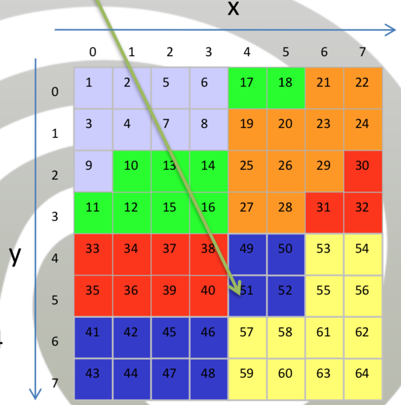
- Z-curve
- Map multidimensional data to one-dimensional values
- Neighboring data - neighboring Z-values
- Z-Value: Bit interleaving of coordinates
- Z-Regions
- Interval on Z-curve
- One disk block
- Efficient processing
- Advantages:
- Provide high node fill degree
- Logarithmic complexity
- Z-curve good performance for range queries
Range query
- Query can be specified by two coordinates (upper left qa and lower right qb)
- RQ-algorithm
- Calculate Z-region of qa (bit interleaving)
- Load block
- De-interleave Z-values
- Check values if in query rectangle
- Jump to next Z-Region in query rectangle
- Repeat 2-5 until last address bigger than qb
- Critical part: How to jump efficiently inside query rectangle?
- Problem: Jumping takes too long, efficiency loss
- Calculation involves bit operations and comparisons
- qa, qb and current Z-Value
Bitmap indexes
- Bit array
- Intended for DW
- Work well if attribute has few distinct values
- Required: Mapping from ID to Block
- Bitmap index for an attribute:
- collection of bit-vectors
- Number of bit vectors = number of distinct values of an attribute
- Length of bit-vector = cardinality of relation
- Advantages
- Operations efficient and easy (HW support)
- Disadvantages
- One bitmap-vector per new value
- Solution: Multi-component bitmap
- Not fit for range queries
- Solution: Range-encoded bitmaps
- One bitmap-vector per new value
Deletion
- Assume record numbers are not changed
- Tombstone replaces deleted record
- Set corresponding bit to zero
Insert
- Inserted record forced appending to all bit vectors
- Inserted record gets next number
- If new records has new value, add new bit-vector
Update
- Change corresponding bit
Select
- Basic AND / OR bit operations
- Use bit-vectors if selectivity is hight
Multi-component bitmap index
- encoding with different numeration system
- \( <3, 4> \) basis encoding
- Advantages
- 100 different days: <10, 10> basis encoding
- Storage reduced from 100 to 20 bitmap vectors
Range-encoded bitmap indexes
- Idea: Set bits of bitmap vectors to 1 if they are higher or equal
- Point query: Two vector reads necessary
- Advantages:
- Bitmap indexes great for indexing dimensions (very small index, smaller than trees)
- Reduce response time for large classes
- Dramatic performance gains
Optimization
Partitioning
- Goal: Flexibility for managing data
- Split data into several physical units
- Key to efficient implementation
- Advantages:
- Inexpensive indexing
- Sequential scans
- Easy recovery / monitoring / reorganization
- Improve:
- Business query performance (minimize data)
- Data availability (backup)
- Database administration
- How?
- Data partitioning (date, geography, …)
- Hardware partitioning (vertical architecture)
Advantages / Disadvantages
- Advantages:
- Group related records together
- Optimize each partition
- Security
- Recovery
- Parallel processing
- Disadvantages:
- Complexity
- Slow retrieval across partitions
Data Partitioning
- Levels: Application + DBMS
- Example Application level: Tax laws for each year
- Types:
- Horizontal partitioning (Rows)
- Vertical partitioning (Columns)
Horizontal partitioning
- General
- Split set of tuples of relation
- Disjoint table parts
- Range partitioning
- Partition key in specific range
- Selection over Master-Relation
- List partitioning
- Partition key is in specific list
- Hash partitioning
- Value of hash function for partition
- Goal: Equal distribution
- Used for parallel processing
- Often used: Time, Table size, Other dim. As time
Vertical partitioning
- Called „row splitting“
- Separate highly and rarely used columns
- Create view for old table
- Maintenance the link: Performance cost
- Special case: Mini-dimensions
- Split dimension table (highly vs. rarely used)
- Must be distinct
- Should be compact/small
- Performance boost (browsing etc.)
Partitioning management
- Goal: Transparent outside DBMS
- DBMS provides Master-Table at logical level
- Data migration
- Records can be updated -> different partition
- Default behavior: error
- Row movement allows update
Join optimization
- Reason: Queries over several partitions
- Joins generally expensive
- Join trees with different costs
- Number of possible join trees: Catalan numbers
Star join
- Star-schema: Big fact table, small dimension table
- If restrictions or group by on n dimensions, n+1 order join necessary
- Goal heuristics: Reduce number of join orders
- OLTP: Don’t join table with no common attribute
- Not suitable for OLAP
- Dimensional cross product can become very large
- DB2:
- B*-Tree index on fact table for each dimensions
- Semi-join on index
Materialized views
- Provide very fast access
- Maintenance expensive
- Store aggregated results
- Other solutions to speed up queries:
- Pre-compute involved joins
- Pre-compute often queries
- Issues:
- Utilization (what to materialize? What indexes?)
- Choice of views (Which views to use for answering?=
- Maintenance (how frequently refresh?)
Utilization
- Should be transparent
- Rewrite queries internally
- Rewrite using query execution graph
Integration
- Valid replacement: Result must be equal
- Finding replacement is NP-complete
- Conditions to integrate view in query:
- Selection in view not more restrictive
- Projektion from query is subset of projection of view
- Aggregation must be possible
- Additional selection must be possible
- Selection in view more restrictive than in query:
- Split query in view and not-view part
Choice
- Static:
- Choice by DBA
- MV from older queries
- Dynamic:
- MV adapts itself to new queries
Static Choice
- Consider „benefit“ of view
- Cost function: Query costs, frequency of query, maintenance costs
- Knapsack problem
- Limited storage
- Algorithm chooses from lattice the cuboid to materialize
- Disadvantages:
- OLAP interactive (user makes ad-hoc queries)
- Queries always changing
- There are often repeating queries that should be materialized
Dynamic Choice
- Monitor queries (calculate benefit)
- Materialized view processing plan MVPP
- Modify MVPP in background
- Decide on views
- Caching with semantic knowledge
- Factors for benefit:
- Frequency
- Size of view
- Number of supported queries
- Access time
Maintenance
- Goal: Keep view up-to-date
- Important: How and when to refresh?
- Naive: Re-computation on every update
- Incremental: Change view by inserted/deleted values
- When to refresh?
- Immediate
- Advantage: Always consistent
- Disadvantage: slow updates
- Deferred
- Advantage: Maintenance without slow updates
- Disadvantage: Inconsistent view
- Refresh
- Lazy (delay until next query on view)
- Periodic (refresh periodically, possible inconsistent but ok)
- Event-based (e.g. after fixed number of updates)
- Immediate
OLAP
DW Queries
- Large amount of data
- Mostly read
- Purpose: Analytics
- OLAP Application:
- Management information (Sales)
- Government (Census)
- Scientific databases (Geo-Informatics)
- Goal: Response time of seconds / few minutes
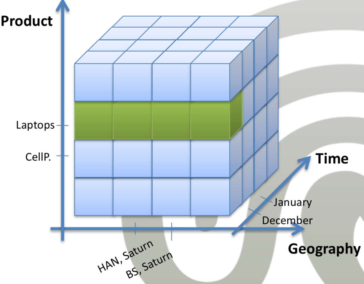
OLAP Operations
- Typical:
- Roll-up
- Drill-down
- Slice
- Dice
- Pivot
- Other:
- Aggregate
- Ranking / comparing
- Drill-across
- Drill-through
Roll-up
- Goal: Aggregation (get generalization)
- Hierarchical roll-up:
- Climb attribute hierarchy (no drop)
- Dimensional roll-up:
- Drop dimensions
- Maximum hierarchical roll-up = Complete dimensional roll-up
Drill-down
- Goal: De-aggregation (high to low)
- Introduce dimensions
- Required: Existence of finer grained data
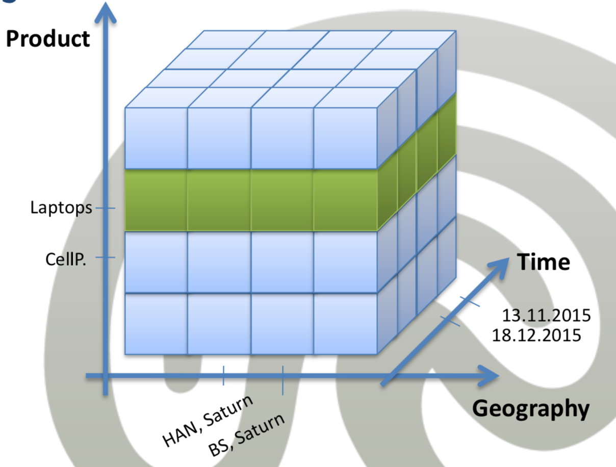
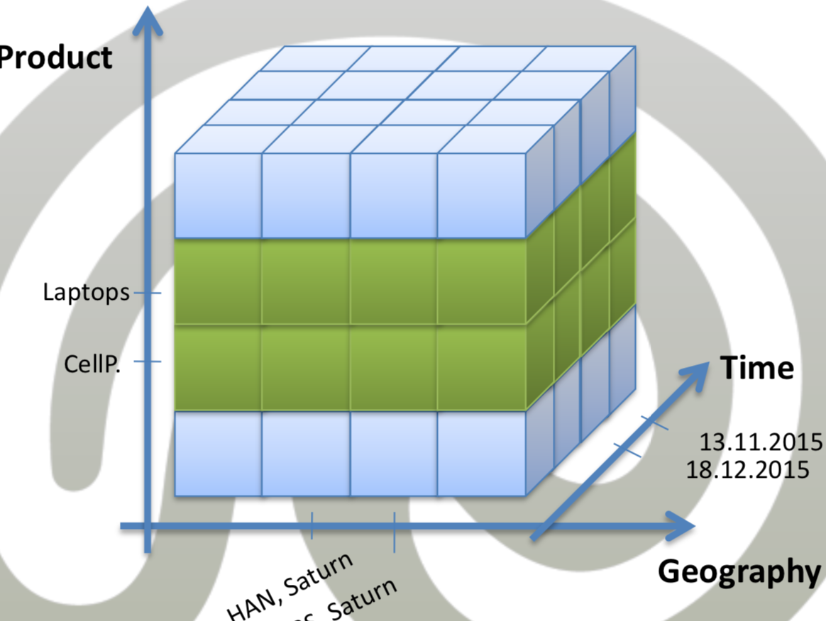
Pivot
- Rotate: Re-arranging data for viewing
- Aggregate measures
- Grid with (x, y) coordinates
OLAP Data Visualization
- Problem: OLAP hard to express in Query language
- -> OLAP Client have GUIs
- Visualization three dimensions
- Layers (like sheets in Excel)
- Nesting (Combined cells)
OLAP Server
- Client: Display reports, allow interaction (OLAP operations)
- Server: Provide requests data (MOLAP vs. ROLAP vs. HOLAP)
- Server:
- high-capacity, multi-user data manipulation engine
- Support multidimensional data
- Server architecture
- Physically save multidim. (MOLAP)
- Simulare multidimensionality (ROLAP)
- Hybrid (HOLAP)
- Queries:
- SQL-99 for ROLAP
- MDX for MOLAP/ROLAP
SQL-92
- Problems:
- Performance
- Limited expressiveness
- Multiple aggregations (-> union multiple queries)
- comparisons with aggregations (-> self-join)
- Reporting features (-> too complex)
- No statistical functions
OLAP Queries
- Select by attribute
- Group by attributes
- Aggregations
OLAP Functions
- Moving average
- Percentile
- Ranks
- Window clause (action over set of rows)
- Partition, order, aggregation
Ranking in SQL
- Row numbering:
- ROW_NUMBER() OVER (subquery)
- Non-deterministic for ties
- RANK / DENSE_RANK
- DENSE_RANK - continuous ranking
- Group ranking
- Partition by
NTILE
- Split set into equal groups
- Divide ordered partition into buckets
- NTILE(4) - quartile
- NTILE(100) - percentage
SQL-99
- New: GROUPING SET, ROLLUP, CUBE, Aggregations, Topk
- GROUPING SET
- (a, b) -> Aggregation by a and by b
- NULL values: Operator returns 0 for „real null“
- ROLLUP
- (a, b) -> Aggregation by (a, b), (a), ()
- CUBE
- (a, b) -> Aggregation by (a, b), (a), (b), ()
MDX
- Multidim. Query language by Microsoft
- ROLAP support -> translate to SQL
- Similar SQL Syntax
- Elements:
- Lists {A, [A B], C}
- Generated elements Germany.CHILDREN
- Functional generation DESCENDENT(USA, Cities)
- Special functions: TOPCOUNT, TOPPERCENT, TOPSUM and filter
XMLA
- Goal: Standardized API for OLAP
- mdXML is MDX wrapper
- Technologies: XML, SOAP, HTTP
ETL Process
DW Project
- Tasks:
- Communication
- Conflict management (magical triangle)
- Quality assurance (Performance, reliability, scalability)
- Documentation
- Project timeline:
- Phase 1: Proof of concept
- Phase 2: Controlled Release
- Phase 3: General Availability
- Most important: ETL
- Software choice:
- Database system (MDB vs RDB)
- ETL tools
- Analysis tools (Data mining vs. reporting)
- Repository
- Hardware choice:
- Data storage (RAID, SAN, NAS)
- Processing (CPUs, SMP, Cluster)
- Failure tolerance (RAID, Mirroring)
- Other factors (Transfer rates, network)
ETL
- Extract - Transform - Load
- Usage: Pull data out of ODS and insert into DW
- Migrate data
- Convert data
- Integrate heterogenous systems
- Balance: Write data / keep data in memory
- Challenges:
- Fast transfer from source to target
- Fault-tolerant (not restart whole process)
- When ETL?
- Periodically
- Refresh policy by DBA
- Different policies for different sources
- Rarely vs. on every update
Staging area
- Data owned by ETL team
- No access (except ETL processes)
- XML Data
- Common format (in- and output)
- Not used for persistent staging
- Relational tables
- Commonly used
- Advantage
- Good metadata
- Relational advantages: Integrity, normalized
- Easy to access
- Disadvantages: Slower
Flat files
- Tools based on Scripting languages
- Advantages
- No overhead
- Sorting/merging/etc. faster outside DBMS
- Disadvantages
- No „updating“
- No index
- Queries/random lookup not supported
- When to use?
- Filtering: grep
- Replacing text: FS-level faster
- Recovery (flat files persistent)
- Sorting (important, FS-level faster)
Data Extraction
- Steps:
- Initial extraction (create logical map)
- Ongoing extraction (new data, changed data)
- Logical map: Connect source and target data
- Data discovery phase (Collect/document source system)
- Anomaly detection phase (dangerous NULL)
- Solve NULL anomalies:
- NULL on foreign key: outer join
- Business rule
- Ongoing extraction
- Maintain DW data after initial load
- Detect changes
- Audit columns
- Database log scraping/sniffing
- Process of elimination
Detect changes
- Audit columns
- Store date/time of change of record
- Detect changes (comparing timestamp)
- Log scraping
- Scan redo log for interesting changes
- Problem: Emptied log
- Log sniffing
- Check log perdiodically
- Better for real-time ETL
- Process of elimination
- Keep copy of previous extraction
- Compare new extraction with old
- Only process differences
- Advantage: Can detect deleted rows, impossible to miss data
Data Transformation
- Use rules, lookup tables, other data
- Goal: Convert data to desired state
- Steps:
- Data Cleaning
- Data integration
Data Cleaning
- Data Quality characteristics:
- Correct
- Unambiguous (only one meaning)
- Consistent (convention)
- Complete (not null)
- Data cleaning engine:
- Data-profiling results (meta-data, quantitative assessment)
- Error event table (error event fact table, star schema, details)
- Audit dimensions (describe data quality for each record, attached to fact table)
Data Quality
- Tools: Oracle Data Profiling, DataCleaner
- Important: Anomaly detection
- Data sampling for large tables
- Data profiling: Analyze outliers
- Data distribution:
- Flat distribution
- Zipfian distribution
- Pareto, Poisson, S-distribution
Data / Schema Integration
- Steps:
- Preintegration analysis
- Comparison of schemas
- Conformation of schemas
- Merging and restructuring
- Semantic process
- (Semi-)automated matching
Pre-integration analysis
- Close look on individual schemas
- Choose adequate integration strategy
- Binary (sequential, balanced)
- N-Ary (One-shot, Iterative)
- Conflicts:
- Table/Table: Naming, structure, constraints
- Attribute/attribute: Naming, defaults, constraints, types
- Table/Attribute
Conformation of schemas
- Goal: Make schema compatible for integration
- Manual interaction:
- semantical resolving
- Renaming
- Converting types
- Aligning cardinalities/functionalities
Schema matching
- Label-based matching (measure semantic similarity)
- Instance-based matching (data-distribution across DB instances)
- Structure-based matching (element types, hierarchies, number/type relationships)
- Query-driven integration: Schema mapping
- Practice:
- Data Translation Tool
- Data Transformation Tool
- OpenRefine
Data Loading
- Types:
- Initial load
- Continuous load
- Issues:
- Huge data volumes
- Small time windows
- When build index/aggregations?
- Recover gracefully
Initial Load
- Deliver dimension tables
- Deliver fact tables (bulk-load features/parallel)
- Tools
Continuous load
- Load over time
- Carefully schedule (maintain integrity, completeness)
- Possible results: Error duplication, inconsistencies
- Steps:
- separate updates from inserts
- Drop any index not required for updates
- Load updates
- Drop all indexes
- Load inserts
- Rebuild indexes
Metadata
- Describe contents of DW and how to use
- Source system metadata
- Source specifications (repositories, schemas)
- Source descriptive information (ownership, access methods)
- Process information (extraction code, job schedule)
- Data staging metadata
- Acquisition information
- Definition of dimensions
- Aggregations (DBMS load scripts, definitions)
- Audit, job logs, documentation, lineage
- DBMS metadata
Real-time DW Motivation
- Company delivering energy
- In-time accuracy enhances business
- Real-time <> fast
- Real-time DW enforces time constraints
- ETL process
- Involves downtime
- ODS to flat files (unavailable for queries)
- Can take hours
- -> Redesign ETL for real-time DW
Real-time ETL
- Solutions
- Microbatch
- Direct Trickle-Feed
- Trickle & Flip
- External Real-time Data Cache (ERDC)
- Microbatch
- classical ETL-batch
- Very small batches
- Provides near-real-time ETL
- Reduce intervals to 3/4 hours
- Requires automized transformation
- Interval depends on: Data volume + ODS/OLAP load
Direct Trickle-Feed
- Continuously insert into DW
- Microbatch with batch-size 1
- Problem: Query contention
- Updating tables being queried
- Performance decreases
- Solution: Separate Rea-time fact partition
- Idea: Separate fact table and new data
- Link two tables seamlessly
- Index the real-time partition lightly (incoming data)
Direct Trickle-Feed: Practice
- Keep 150 MB real-time partition in memory
- Query answering
- Query processor analyzes query
- Send to real-time partition and static fact table
- Benefit: Index of fact table, small size of in-memory partition
- Query contention still possible
Trickle & Flip
- Insert data into staging table
- Format is exact the format of the fact table
- Halt trickle, copy staging table, switch pointers
- -> ETL paused, OLAP can continue during copying
- Problem: Scalability
- Staging table must contain complete fact table
- Refresh frequency ~ Flip duration
- -> Copying very slow
- Advantage: No query contention (flipping very fast)
ERDC
- Store incoming data outside DW (avoid performance problems)
- Separate & isolate querying:
- Route real-time data queries to ERDC (No scalability problem)
- Assumption: Real-time volume small
- Load data regularly into DW
- Problem: Can’t join real-time and historical data
ERDC - JIM
- Just-in-Time Merge
- Extension of separate & isolate
- Pre-process query: Identify real-time data parts (attrs/rows)
- Load snapshot from ERDC into DW
- Re-write query to include real-time data
- Advantages:
- Less scalability problems (real-time data only on request)
- No query contention (no change while querying)
- Problem: Very complex query processor, Not supported
Real-time ETL Decision
- Decision depends on application!
- Microbatch: Easy/cheap for near-real-time (3-4 h)
- Direct Trickle-Feed
- Real-time performance
- Normal daily data load
- Query contention (large number of users, complex OLAP)
- Trickle & Flip: near-real-time performance (delay because of copying fact table)
- ERDC + JIM
- True real-time performance
- Rapidly changing data
- Concurrent access hundreds of users
- Joining real-time + historical data
OLAP on changing data
- OLAP
- unchanged, static, historical data
- no precautions for consistency
- Problem: OLAP on changing data -> inconsistent results
- 10-50 passes
- Range from seconds to hours
- Inconsistencies most probable + problem for real-time DW
- Inconsistency problem not affects:
- Microbatch, Tricke & Flip
- Fresh copy of data, no refresh during OLAP
- ERDC+JIM: External data read-only during query
- Microbatch, Tricke & Flip
Hybrid OLAP/OLTP
- OLAP too long to execute
- OLTP locked while performing OLAP
- Idea: Shadow OLTP data, run OLAP on shadows
- avoid inconsistencies
- Limited by hardware (too slow)
Storage
- Properties
- Random access time: avg. time access random piece of data
- Transfer rate: avg. amount of data per minute
- Volatile: Need power to keep data (static/dynamic)
- Access modes: Random/Sequential
- Storage hierarchy:
- Primary storage: frequent used data (fast, expensive, limited capacity)
- Secondary storage: Main stored data (slower, large)
- Tertiary storage: Backup (Huge capacity, cheap, offline)
SSD
- Non-volatile memory chips
- Memory: Wears down, non-volatile
- Controller: Error correction, wear leveling, bad block mapping
- Advantage: Silent, shock resistant, low access time
- Disadvantage: Write amplification, Limited rewrite ability
- SSD-based DW:
- Advantage: 10x faster than HDD, persistent
- Disadvantage: Not fast enough, Wears down (not suitable for OLTP)
RAM
- Dynamic Random Access Memory (DRAM)
- Volatile RAM
- Sometimes internal battery: persistence
- Ultrafast access
- Expensive
- DRAM-based DW:
- Very high access speed (2000x fast than HDD)
- Problem: No power -> data lost
HyPer
- Hybrid OLAP/OLTP main memory database
- Goal:
- Process OLTP very fast
- Process OLAP on up-to-date snapshots
- OLTP Processing
- Process queries sequentially
- No IO
- 10000 tps
- Multi-thread OLTP processing
- parallelize reads
- Locks for insert/updates/deletes
OLAP
- Problem: Query contention
- Solution: Run OLAP on snapshots
- Snapshot management
- Create virtual memory snapshot
- Fork system call
- Parent/child share memory
- Uses copy-on-write (only changed data copied)
- Shadow data through pointers
- OLTP change -> copy value to OLAP page
SAP HANA
- Real-time business intelligence in-memory
- OLTP: Rows store
- OLAP: Column store