Distributed Databases

General

• Distributed Database keeps all features of a centralized database
• Restrictions
  • Limited scaling (rarely scale over 50 nodes)
  • Limited flexibility (fixed schemas, lot of manual work)
  • High administration costs (adding/removing nodes)
  • High hardware costs (specialized/reliable hardware)
• Nice-to-have features
  • Unlimited linear scaling (performance + storage capacity)
  • Flexible schema (support schema change)
  • Elastic computing (adapt available resources)

Applications of DDBMS

• Astronomy
  • Store telescope images at site
  • Increasing storage requirement due to improved technology
  • Information is dynamic
  • Information is multi-typed (e.g., image, time series, spectra)
  • Provenance required (i.e., know all details)
• Military
  • Data: Sensor data, geographic data, technical information, …
  • Interactive: Annotate/extend given data
  • Requirements:
    • Consistent/real-time-view
    • High reliability
    • Many write operations
  • Use ACID

Motivation

• Scenario: Company has branches of different continents (distributed scenario)
• Additional/new requirements:
  • Data-integration (e.g., cross-branch transaction)
  • Resource sharing (e.g., use existing hardware efficient)
  • Failure resilience (e.g., disaster resistant)
  • IT Infrastructure should reflect company structure
• Possible solutions
  • Integrate multiple DBMS
  • One DMBS on multiple nodes

Definitions

Distributed Database

A Distributed database is a DB (DDB) where data is store on several nodes in a network.

Distributed DBMS

A Distributed DMBS (DDBMS) is a DMBS managing several data nodes.

Classification and different types

• Classification criteria
  • Autonomy (degree of coupling of nodes)
  • Heterogeneity (DDBMS used)
  • Transparency (schema, query, update)
• Types
  • Homogeneous DDB
    • Regular DDB
    • Parallel DDB
  • Heterogeneous DDB
    • Multi Database
    • Mediator Database
    • Federated Database

Homogeneous DDB

• One DDBMS
• Each node controlled by same DDBMS
• Globally shared schema
• Types
  • Regular DDB
  • Parallel DDB

Regular distributed database

• Nodes
  • Linked by slow WAN
  • Semi-autonomous
• Manual data distribution (distribution because of different locations)
• Examples
  • Banking/insurance company

Parallel distributed database

• Nodes
  • Linked by high-speed LAN
  • No autonomy
• Automatic data distribution
• Examples
  • High-performance data center

Heterogeneous DDB

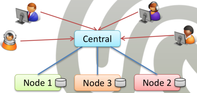
• Goal: Present unified query interface
• Each node autonomous
• Each node can run any centralized DBMS
• Central node passes queries to nodes
• Types
  • Multi Database
  • Mediator Database
  • Federated Database
• Disadvantage
  • Query rewriting during runtime (expensive)

Multi database

• Use case: Mergers and aquisitions
• No integration between nodes
• No shared schema/view
• Central node tasks
  • Data retrieval from nodes/data integration
• Advantage
  • Complete query scope of all nodes
• Disadvantage
  • Complete integration on user side

Mediator database

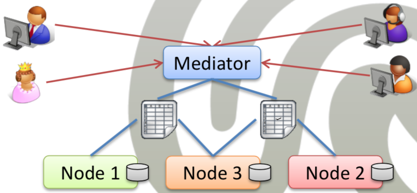
• Use case: Provide view on nodes
• Central node is called mediator
  • Mediator provides shared views to clients (subset of data)
  • Mediator maps queries to individual schemas and creates result
• Examples
  • Distributed bio/chemical database
• Advantage
  • Integrate only necessary tables
• Disadvantage
  • No write access
  • Query only subset of data

Federated database

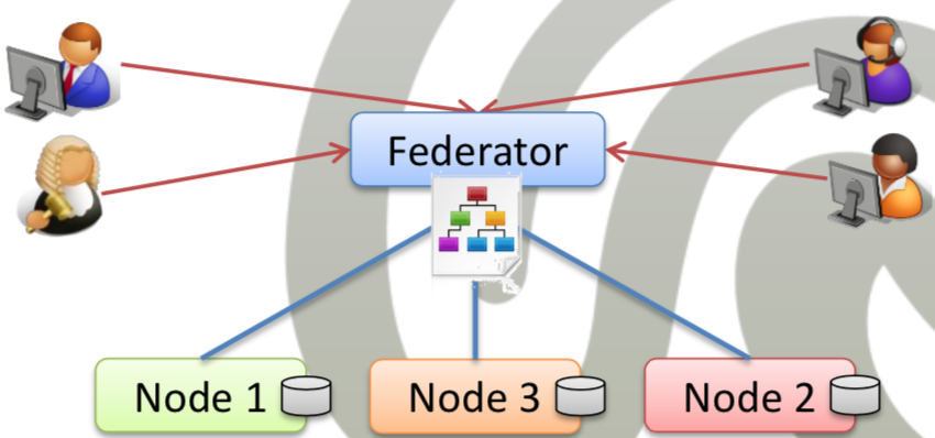
• Central node is called federator
• Federator provides globally shared schema
• Federator maps queries to individual schemas and creates result
• Examples
  • Big cooperate database system
• Advantage
  • Users can write into tables
  • Schema transparency
• Disadvantage
  • Complex integration

Transparency

Schema transparency

• DDBMS automatically distributes data
• Automatic sharding
• Advantage
  • No consideration of distribution
• Disadvantage
  • No usage of semantic knowledge (locality)
  • High-speed network required

Query transparency

• Querying: user doesn’t need any knowledge about data location
• Advantage
  • Easy querying (like single-node DBMS)
• Disadvantages
  • Distributed query optimizer required
  • Statistical data on nodes required

Update transparency

• Updating: user doesn’t need any knowledge about data location
• Advantage
  • Global consistency ensured
  • Easy updating
• Disadvantage
  • Complex (distributed transaction manager required)

Sharing architectures

General

• Classification of distributed architecture based on sharing
  • Shared secondary storage (HDD, RAID, SAN)
  • Geographic location
  • Main memory (i.e., node coupling)

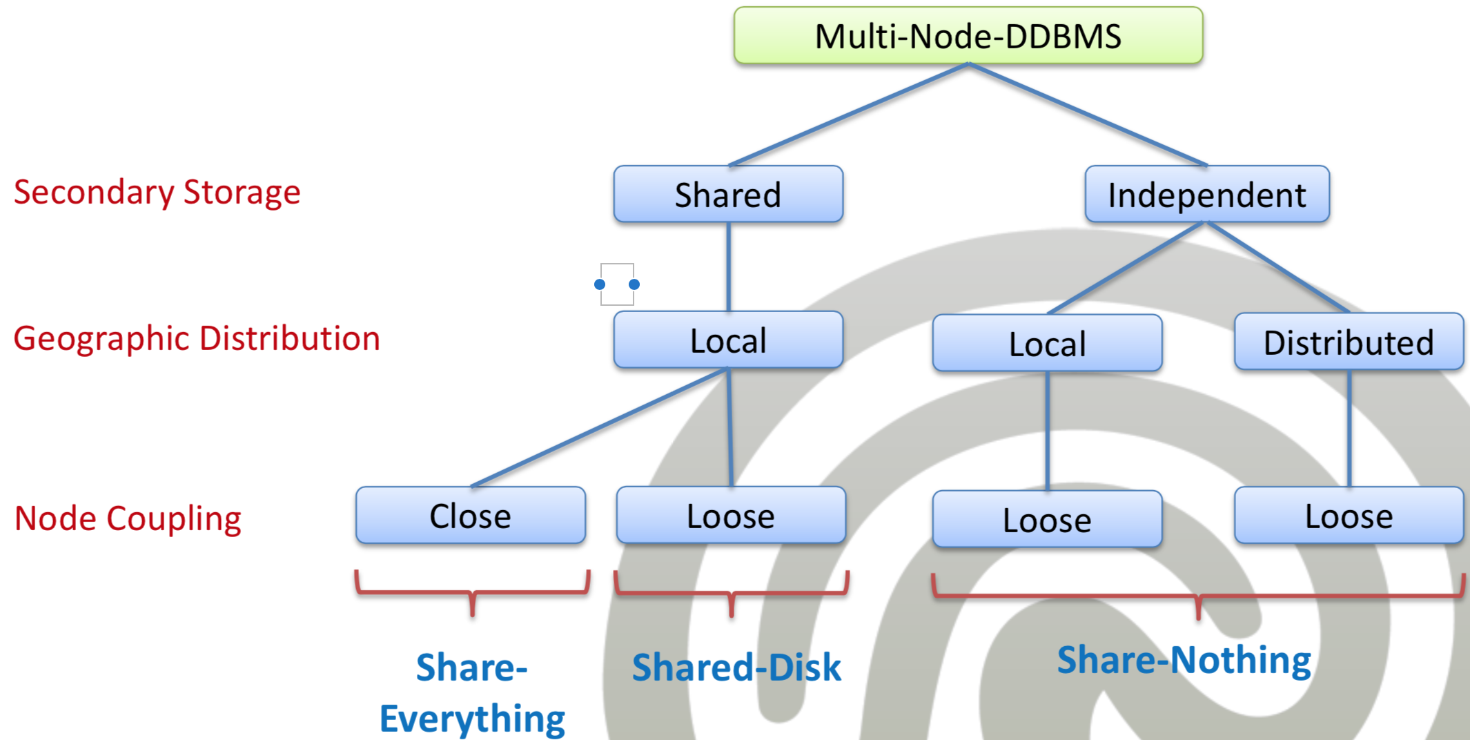
Definitions

• Node
  • Single computational device (computer, server, CPU)
• Node group
  • Logical group of nodes
  • Sharing an agenda
• Site
  • Group of nodes in the same location
  • Connected with high-speed network
  • Node in exactly one site

Share-Everything

• Shared main memory
• Shared secondary storage
• Problems
  • Scalability (main memory bottleneck; capacity, locks, latches)
  • Reliability (Main memory Single Point of Failure)
• Technologic improvement
  • Massively parallel computer cluster
    • Used to implement high-performance parallel DDBMS
  • Remote direct memory access RDMA
    • Nodes have own memory
    • Access memory of other nodes via low-latency high-performance network
    • NUMA architecture
• Major shared-everything architectures
  • Symmetric multiprocessor system (SMP)
  • Non-uniform memory access (NUMA)

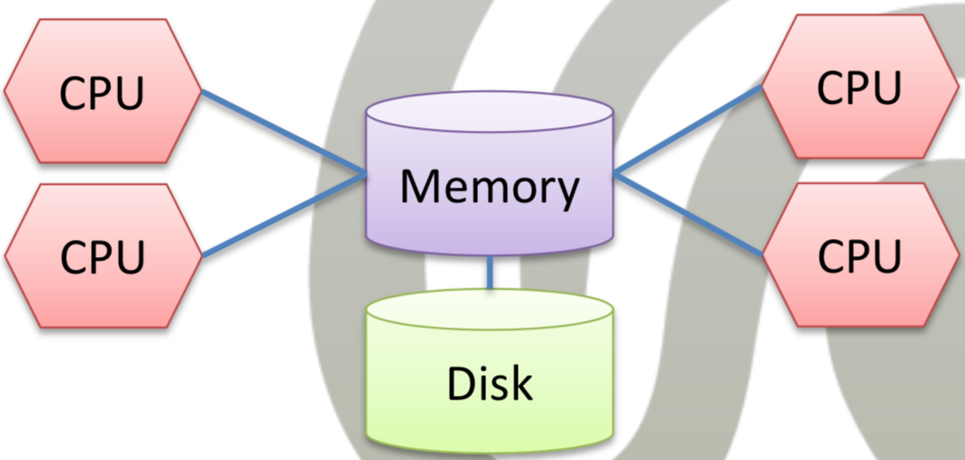
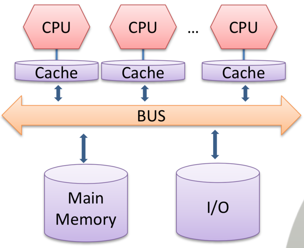
Symmetric multiprocessor system

• Architecture
  • Centralized main memory
  • Shared with multiple homogeneous processors
  • Central control for processors
  • Each processor
    • Own cache
    • Central bus connecting to I/O and disk
• Advantage
  • Any processor can do any task
  • Good load balancing
• Disadvantage
  • Bus becomes bottleneck
  • Processor can block cache (called cache coherency, in NUMA not that much)

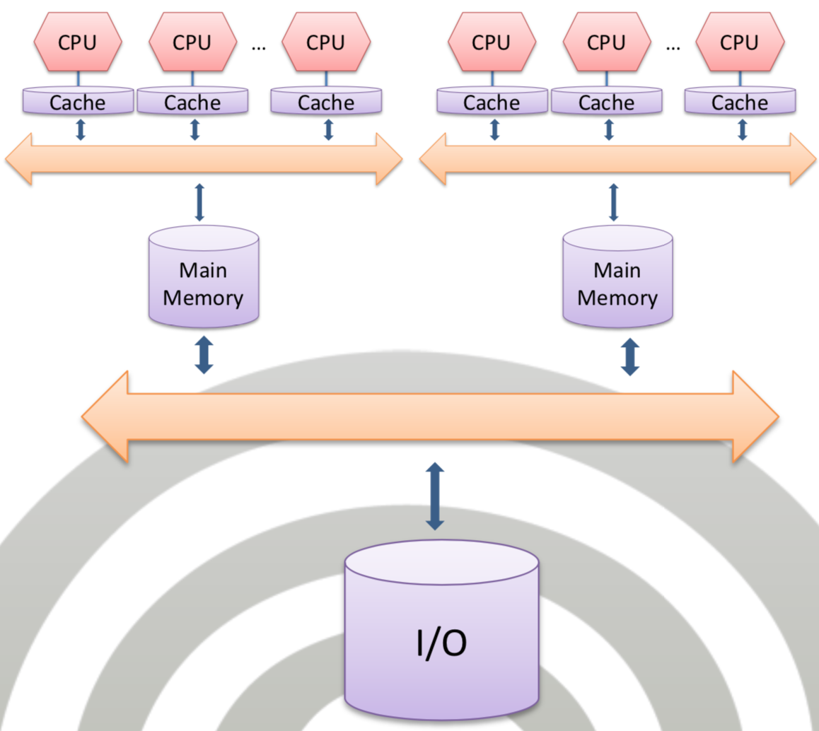
Non-uniform memory access

• Architecture
  • Partitioned main memory
  • Complete memory can be accessed
  • Close memory can be accessed more efficiently
• Advantage
  • If efficient partitioning, good scalability
• Disadvantage
  • Requires careful partitioning of data

Share-Disk

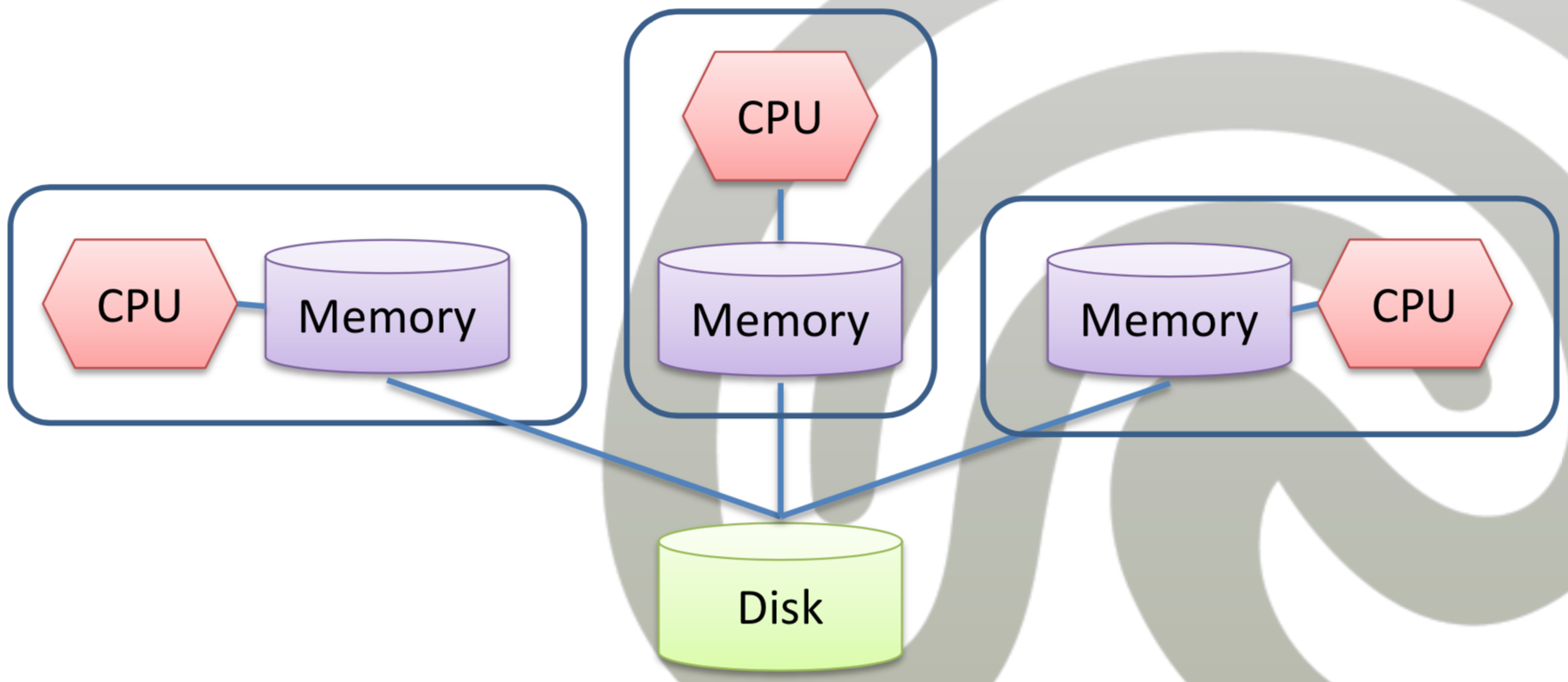
• Shared hard disk
• Query processing: Use intermediate results on hard disk
• Common for enterprise level DDBMS
• Data stored in high-performance SAN

Share-Nothing

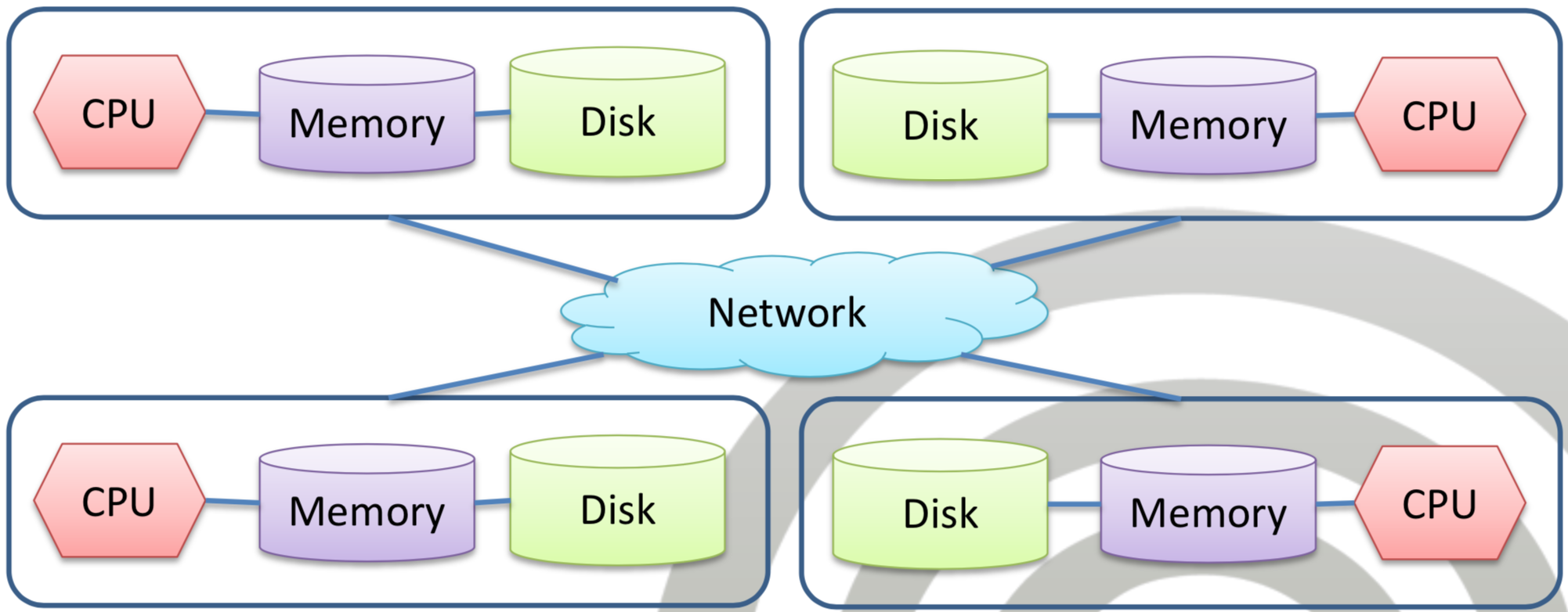
• No shared storage/memory
• Communication over network
  • Can result in high shipping costs
  • If no shipping is necessary, system is linear scalable

Data distribution

General

• Two major issues
  • Fragmentation (split relations into chunks)
  • Allocation (assign fragments to nodes)
• Describe fragmentation and allocation as minimization problem
  • Minimize execution costs
    • Minimize query costs
    • Minimize update costs
    • Maximize parallel access/execution (load balancing for multiple nodes)
    • Minimize communication costs (necessary data should be local)
    • Maximize availability
      • High geographic distribution
      • High replication
      • Data should be near by client
      • Data should be resilient to (site) failure
  • Use information on app/data
    • For Fragmentation: Qualitative data (query predicates, schema)
    • For Allocation: Quantitative data (query location, query load, selectivity)

Fragmentation

General

• Fragmentation considers the
  • Splitting of relations (chunks)
  • Size of fragments
• Intuitive heuristic
  • Fragments should contain data which is accessed as unit
  • e.g. horizontal partitioning: Query predicates
• Bad designed fragments
  • Performance problem
• Defintion Partitioning
  • Fragment is stored only once
• Partitioning techniques
  • Horizontal partitioning
  • Vertical partitioning
  • Hybrid approaches
• Correctness rules
  • Completeness rule (no data is lost)
  • Disjointness rule (Fragments do not overlap)
  • Reconstruction rule (fragmentation preserves data and properties; constraints, keys, attributes)

Horizontal partitioning

General

• Idea
  • Relation is split horizontally
  • Distribute tuples
• Techniques
  • Range partitioning
  • Value lists
  • Hash values
• Correctness rules
  • Horizontal completeness rule
    • \( R = \bigcup R_i \)
  • Horizontal disjointness rule
    • \( \forall i\neq j: R_i \cap R_j = \empty \)
  • Horizontal reconstruction rule
    • Primary keys remain unique
    • Preserve foreign keys
• Types
  • Primary Horizontal partitioning
    • Hash-based partitioning
  • Derived Horizontal partitioning

Primary Horizontal partitioning

• Create fragments by selection operation
• \( R_i = \sigma_{P_i}(R), 1\leq i \leq n \)
• Find predicate \( P_i \)
  • Manually
  • Automatically at design time
  • Automatically at runtime
• Manual primary horizontal partitioning
  • DBA uses semantic knowledge (e.g. by regions)
• Automatically at design time
  • Common approach
  • Estimate query frequency/load of common queries
  • Compute optimal fragmentation (often hash-partitioning)
  • Issue: Static schema
• Automatically at runtime
  • Automatically adapt to usage statistics
  • No administrative input (supports elasticity)
  • Difficult (often used with simple data model, e.g. Cloud)

Automatically at design time: Minterms

1. Define queries and their frequencies
2. Rewrite selection conditions into disjunctive normal form
3. Extract set of minterms
   • Definition: Terms only using negation and conjunction
4. Estimate selectivity of each minterm
5. Find minimal and complete sets of minterms
   • Definition minimal: At least one query access fragment
   • Definition complete: Access probability for each tuple in a fragment is similar
6. Define fragments

Automatically at design time: Hash-based partitioning

• Also used in peer-to-peer systems
• Idea
  • Create hash for tuple
  • Each node responsible for one range
• Advantage
  • Automatic partitioning
  • No semantic knowledge necessary
  • Easy load balancing (uniformly distributed load)
  • Easy implementation
  • Stable performance
• Disadvantage
  • No semantic knowledge (performance may suffer)
  • Ignores query load

Derived Horizontal partitioning

• Motivation
  • Reconstruction rule states that foreign key dependencies must be preserved
  • If a relation with foreign keys is fragmented, the corresponding relation should be fragmented, too
• Use Join link graphs
  • Link is a foreign key dependency
  • Owner relation: Source
  • Member relation: Target
• Formal problem
  • Relations \( R, S \)
  • Foreign key link from \( S\rightarrow R \)
  • \( S \) is partitioned in \( S_1,...,S_n \)
  • Partition \( R \) w.r.t \( S \)\( R_i := R \ltimes S_i, 1\leq i\leq n \)
• Problems
  • Incomplete fragments (\( R \) contains \( NULL \) values)
    • Solution: Put into one fragment
  • Overlapping fragments (Foreign key from \( R \) to \( S \) on non-unique attribute and \( S \) is fragmented by another attribute)
    • Solution: Fragmentation on foreign key
  • Multiple dependency links (\( S\rightarrow R, T\rightarrow R \))
    • Solution: Most-used relation + best join characteristics
• Good join characteristics
  • Small fragments
  • Locality (join executed on single node)
  • Use Fragment Join Graphs
    • Node: Fragment
    • Link: Foreign key dependency
    • The fewer links, the better
    • Best case: Simple join graphs
    • Worst case: Fully-connected graph

Vertical partitioning

• General
  • Split relation vertically
  • Distribute columns
  • Replicate primary keys
• Correctness rules
  • Vertical completeness rule (each attribute in one fragment)
  • Vertical disjointness rule (each non-primary-key attribute in exactly one fragment)
  • Vertical reconstruction rule (\( R=R_1\bowtie ... \bowtie R_n \))
• Formal
  • Attributes for fragments \( A_R=\{A_1,...,A_n\} \)
  • Fragments \( R_i = \pi_{A_i} R, 1\leq i \leq n \)
• How to find fragments?
  • Possible combinations
    • \( m \) non-primary-key attributes
    • \( B(m) \) possible fragmentations
    • \( B(m) \): m-th Bell number (number of partitions of \( m \) elements)
  • Use heuristics
    • Grouping heuristics (fragment for each non-primary-key attribute, then join for given criteria, bottom-up)
    • Splitting heuristics (relation is one fragment, split until criterion, top-down, better performance)
  • Goal: Fragments contain attributes accessed together
  • Idea: Find attributes that are queried together (use statistics)
• Pareto principle
  • 20 % of queries produce 80 % of load (power law)

Attribute Usage Matrix

1. Find typical queries
2. Create query-attribute incidence matrix \( A_{use} \)

Attribute Affinity Matrix

1. Get query statistics vector \( q_{stat} \)
2. Create matrix \( Q_{stat} = diag(q_{stat}) \)
3. Compute attribute affinity matrix \( A_{aff} = A_{use}^T * Q_{stat} * A_{use} \)
   • Which attribute is queried with which attribute how often together?
4. Cluster matrix
   • Permute rows&columns to get similar elements closer together
   • Bond energy algorithm
   • Maximize \( \sum_{i=1}^n \sum_{j=1}^n A_{i,j} * (A_{i,j-1}+A_{i,j+1}+A_{i-1,j}+A_{i+1,j}) \)
   • Complexity \( O(n^2) \) (\( n \) attributes)
5. Result: Clustered attribute affinity matrix

Hybrid partitioning

• Combine horizontal and vertical partitioning

Allocation

• Allocation considers the
  • Assignment of fragments to nodes
  • Replication of fragments on nodes
• Replication
  • Advantages
    • Read-only queries executed parallel
    • Reduced communication costs
    • Resilience to system failures
  • Disadvantages
    • High update costs
    • Increased storage
    • Consistency is more complex
• Use partial replication
  • Estimate query/update-ratio for fragments
  • Estimate query load
  • Use network topology / latency
• Allocation strategy
  • Focus on high availability
  • Performance vs. replication

| | Full replication | Partial replication | Partitioning | |:–|:–|:–|:–| | Query processing | Easy | Difficult | Difficult | | Directory management | Easy | Difficult | Difficult | | Concurrency control | Moderate | Difficult | Easy | | Reliability | Very high | High | Low | | Parallel query potential | Very high | High | Moderate | | Parallel update potential | Very low | Moderate | High | | Applicability | Possible | Realistic | Possible | | Storage efficiency | Very low | Moderate | Very high |

Distributed query processing

• Central questions
  • How does distributed query processing work?
  • How to localize the required data for the query?
  • How to estimate response time to select a good query plan?

Fundamentals

• Objectives for DQP are not well-defined
  • Minimize resource consumption (?)
  • Minimize response time (?)
  • Maximize throughput (?)
• Problems
  • Cost-based optimization difficult
    • Network statistics vary (model, shipping)
    • Response-time models (how to estimate?)
    • Costs are unpredictable
    • Quality-of-service agreements
  • Extend physical relational algebra (sending/receiving)
  • Data localization (where is data stored?)
  • Data/structural heterogeneity
• Result: Query optimization is adaptive
  • Optimize query with directly measures information
• Example calculation
  • Tuple access cost \( c_{acc} = 1 \)
  • Tuple transfer cost \( c_{trans} = 10 \)
  • Options: Transfer intermediate results or transfer all data to executing node
• Requirement for optimization: Meta data

Meta data

• Contained inside catalog
• Catalog contents
  • Database schema (tables, views, constraints, keys)
  • Partitioning schema (reconstruction rules)
  • Allocation schema (data location, replication)
  • Network information (node connection, network model)
  • Physical information (indexes, statistics, hardware)
• Central question
  • Where to store catalog?
  • How to store catalog?
• Easy approach
  • Centralized meta data (one node)
  • Options
    • Replicate catalog (small catalog, few changes)
    • Caching (replicate only parts, accept inconsistencies)
    • Fragment catalog (large/often changing catalog)

Optimization

• Central question
  • What should be optimized?
  • When should be optimized?
  • Where should be optimized?
• Assumption: Usage of prepared statements (also called canned queries)
• Types
  • Full compile-time optimization
  • Full dynamic optimization
  • Semi-dynamic optimization
  • Hierarchical optimization
    • Global-local plans
    • Two-step plans

Full compile-time optimization

• Compute full query execution plan at compile time
• Advantage
  • Query can directly be executed
• Disadvantage
  • Outdated (statistics vary, e.g. network and machine load)
  • Many unknown statistics (node statistics)

Full dynamic optimization

• Optimize query at runtime
• Requires
  • Heuristics
  • Learning algorithms
  • Luck
• Advantage
  • Can produce good plans
  • Usage of current information
  • Usable for ad-hoc queries
• Disadvantage
  • Can be unpredictable (heuristics may fail)
  • Complex algorithms/heuristics

Semi-dynamic optimization

• Hybrid approach of compile-time and dynamic optimization
• Pre-optimize query
• While executing the query, monitor behavior (e.g. response time, network properties)
• If deviations occur, compute new plan for missing parts

Hierarchical approaches

• Create plans in multiple stages
• Global-local plan
  • Two plans: High-level + low-level plan
  • Global query plan
    • Create by global query optimizer
    • Task: Focus on data transfer (where to create intermediate results, what to ship)
  • Local query plan
    • Create by individual nodes (centralized query processing)
    • Task: Query plan, algorithms, indexes
• Two-step plans
  • Two plans: Compile time + execution time
  • Compile-time plan
    • Create stable plan (join order, join methods, access paths)
  • Execution-time plan
    • Create dynamic plan (node selection, transfer policy)
    • Use fresh statistics

Data Localization

• Central questions
  • How to reconstruct relations?
  • Where to execute query?
• Problem
  • User queries a global schema
  • Relations are fragmented and allocated to nodes
• Assumptions
  • Fragmentation by partitioning rules (selection + projection)
  • No replication
  • Fragmentation rules stored in catalog
  • Fragment locations stored in catalog
• Basic idea
  • Query rewriter replaces relations with a localization program
  • Use reduction techniques to simplify the localization program (remove unnecessary fragments)
• Notion
  • Query is called generic if the localization program reconstructs the full relation (i.e., the reconstruction rule, \( R=\bigcup R_i \))

Reconstruction

Reduction Rule 1

• Reduction rule/technique for primary horizontal partitioning
• Formal
  • Relation \( R \)
  • Fragments of \( F_R=\{R_1,...,R_n\} \) with \( R_i=\sigma_{P_i}(R) \)
  • Query selection \( \sigma_{P_s} \)
• Idea: Omit empty fragments \( \sigma_{P_s}(R_i)=\empty \)
• The rule
  • \( \forall x\in R: \neg (P_s(x)\land P_i(x)) \Rightarrow \sigma_{P_s}(R_i) = \empty \)

Reduction Rule 2

• Reduction rule for joins in primary horizontal partitioning
• Requirement
  • Relationship partitioning over the join attribute
• Base idea
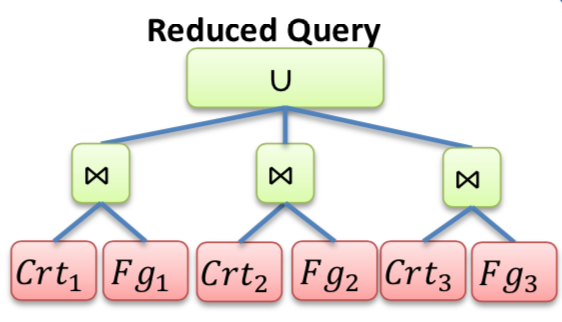
  • Replace large join with multiple partial joins
  • \( (R_1\cup R_2)\bowtie S = (R_1\bowtie S)\cup (R_2\bowtie S) \)
  • Remove empty unions
  • Depends on application if useful
• Optimal case
  • Many partial joins with empty results (requires good partitioning conditions)
  • Many joins on small relations (lower costs)
  • Parallel execution of small joins (could decrease response time, could increase communication costs)
• The rule
  • \( \forall x\in R_i, y\in R_j: \neg(P_i(x)\land P_j(y)) \Rightarrow R_i\bowtie R_j =\empty \)
• Derived horizontal fragmentation is easy
  • Exactly one matching fragment
  • Small number of fragment joins
  • Good for one-to-many relationships

Vertical fragmentation

• Localization program: \( R=R_1\bowtie R_2 \)
• Important: Do not join unnecessary attributes

Hybrid fragmentation

• Localization program: \( R=(R_1\cup R_2)\bowtie R_3 \)
• Guidelines
  • Remove empty relations (reduction rule 1)
  • Remove useless relations (unused attributes)
  • Break/distribute joins (eliminate empty joins)

Execution location

• Central question: Where to execute optimized queries?
• Assumption: Client-server setting
• Approaches
  • Query shipping (thin client)
    • Common approach for centralized DBMS
    • Send query to server
    • Server sends result
  • Data shipping (fat client)
    • Query computed on client
    • Server sends necessary data
  • Hybrid shipping
    • Send partial query to server
    • Send intermediate results to client
• Generalization for multiple nodes possible
  • Query optimizer must decide what/whether to ship
  • Complicated cost model
  • Effective for load balancing
  • Avoid expensive communication

Response time models

• Possible requirements for DDBMS
  • Optimize total resource consumption
    • Classic DB
    • Advantage
      • Good results for heavy computational load
      • Many parallel executions
  • Optimize total response time
    • Waste resources
    • Use fast connections
    • Use intra-query parallelism (parallelize one query)
• Models
  • First tuple
  • Full result
• How to compute?
  • Sequential execution parts (sum of all parts)
  • Multiple parallel threads (maximal costs)
    • Important question: How much speedup is possible?

Amdahl’s Law

• By Gene Amdahl in 1968
• Algorithms are composed of parallel/sequential parts
• Sequential code limit speedup
• \( p \) parallel threads
• \( s \) is fraction of single-threaded code
• \( maxspeedup \leq \frac{p}{1+s(p-1)} \)
• \( maxspeedup = \lim\limits_{p \to \infty}\frac{p}{1+s(p-1)}= \frac{1}{s} \)
• Result: Eliminate all sequential bottlebecks

First Tuple Response

• Central questions
  • How to speed up joins?
  • How to reduce communication costs when sending tuples?
• Improve with pipelining
  • Pipelining
    • No intermediate results
    • Tuple flow
    • Iterator interface is used
    • Useful for scan, select, project, union, join, intersect
  • No pipelining
    • Complete each operation
    • Intermediate results are created (expensive!)
• Problem: Unpipelined join
  • Unsuitable: Block-nested loop join
  • Centralized database: Fully pipelined join unnecessary (one I/O)
  • Distributed database: Fully pipelined join necessary (multiple nodes)
• Solution: Use pipelined joins

Single-Pipelined-Hash-Join

• Join \( A\bowtie B \)
• \( A \) is pipelined
• \( B \) is intermediate result
• \( B \) is stored in hash table (hashed on join attribute)
• Workflow
  1. Hash incoming tuple \( t_A \) from \( A \)
  2. Check against all tuples in bucket \( h(t_A) \) in \( B \)

Double-Pipelined-Hash-Join

• Join \( A\bowtie B \)
• \( A \) and \( B \) pipelined
• Idea: Dynamically create hash table for \( A \) and \( B \)
• Tuple processing on arrival
  1. Hash tuple
  2. Insert tuple in corresponding hash table
  3. Compare tuple against the tuples from the other table
• Issues
  • Balance between \( A \) and \( B \)
  • Use statistics for balancing

Tuple batching

• Problem: Sending each tuple costs too much
• Communication costs
  • Create communication channel
  • Create message
  • Transmit message (header + payload)
  • Receive message
  • Decode message
• Solution: Tuple batching
• Send bulk-messages with multiple tuples
• Pipeline-iterators need cache
• Big batch size (higher than network packet size)

Distributed transaction management

General

• Central questions
  • How to handle transactions if operations are distributed over several nodes?
• Problems
  • Transactions run longer (slow network)
  • Transactions span multiple nodes
  • More possible sources for failure (node, connection, message)
  • No global time
  • Agreement (multiple nodes in one transaction, how to agree?)
  • Consistency (necessary if replication)
• Types of consistency
  • One-copy equivalence (all copies identical values)
  • Eventual consistency (replicas may diverge)
• Handle distributed transactions
  • Central controller (homogeneous DDB)
  • Mediator layer (heterogeneous DDB)

Central controller

• Case: Homogeneous DDB
• Central controller node as transaction manager
• Tasks
  • Grand/release locks
  • Generate schedule
  • Abort/commit transactions
• Requirement
  • Full access to node system resources

Mediator layer

• Case: Heterogeneous DDB
• Idea: Delegate responsibility to local DBMS’
• Use a middleware transaction manager (mediator layer of DDBMS)
  • Supervise execution

Nested transactions

• Idea
  • Split transactions into transaction spanning one node
  • Results in transaction trees
  • Assumption: Node handles transaction locally
    • Advantage: Good if sub-transactions are independent
    • Disadvantage: No real parallelism
• Task of the transaction manager
  • Moderate execution
  • Alone decision on final commit or rollback

Execution

• Execute transaction tree
• Start at root (central node)
• Start child transactions recursively
  • Independent child transactions: Execute parallel
  • Dependent child transaction: Execute sequentially
• Handle failures
  • Abort/rollback all other child transactions
  • Propagate to root
• Scenarions
  • Assume no network/node failures (one-phase commit protocol)
  • Assume network/node failures (two-phase commit protocol)

One-phase commit protocol

• Assumption: No communication/node failures
• New messages
  • Vote-begin
  • Vote-commit
  • Vote-abort
• New states
  • Ready-to-commit
• Single phase: Voting phase
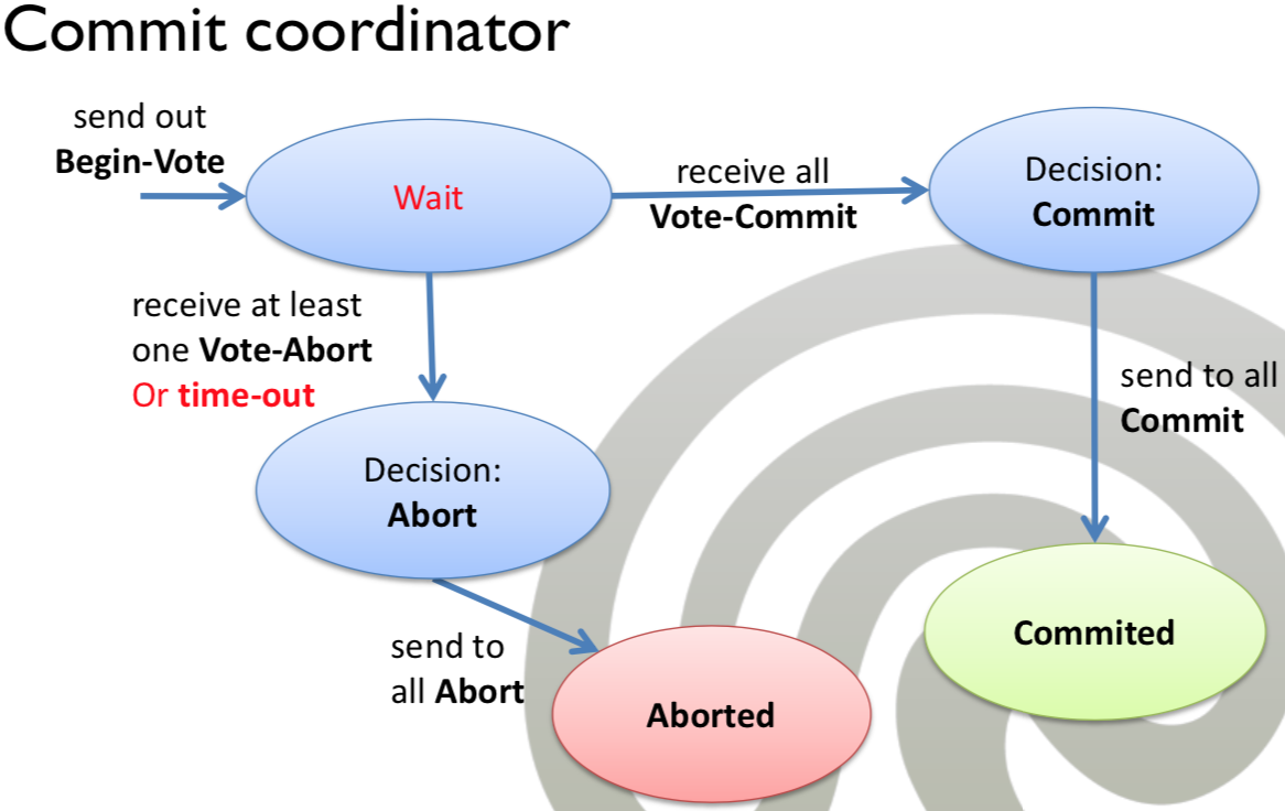
• Commit coordinator
  • Exactly one node is commit coordinator
  • Task
    • Decide about global commit/abort
    • Initiate voting phase
  • If receives one vote-abort, abort all
• Participant nodes
  • Decide bindingly about local commit/abort
  • Send vote-abort or vote-commit
  • Use redo/undo logging (abort and commit are possible)

Two-phase commit protocol

• Assumption: Communication/node failures
• Goal:
  • Create consensus in synchronous replication
  • Ensure atomicity
• Often used together with D-2PL
• Two phases
  • Voting phase
  • Decision phase
• New messages
  • Time-out
  • Help-me
• New states
  • Recover
  • Blocked
• Voting phase
  • Coordinator
    • If coordinator does not receive at least one message or time-out, global abort
  • Participant
    • If participant does not receive a message (time-out), go into state recover and send help-me to participants and wait (state: blocked)
    • If a participant has committed, commit
    • If a participant has aborted, abort
    • If a participant has not voted, the participant sends vote-abort
    • If a participant ready-to-commit, no solution

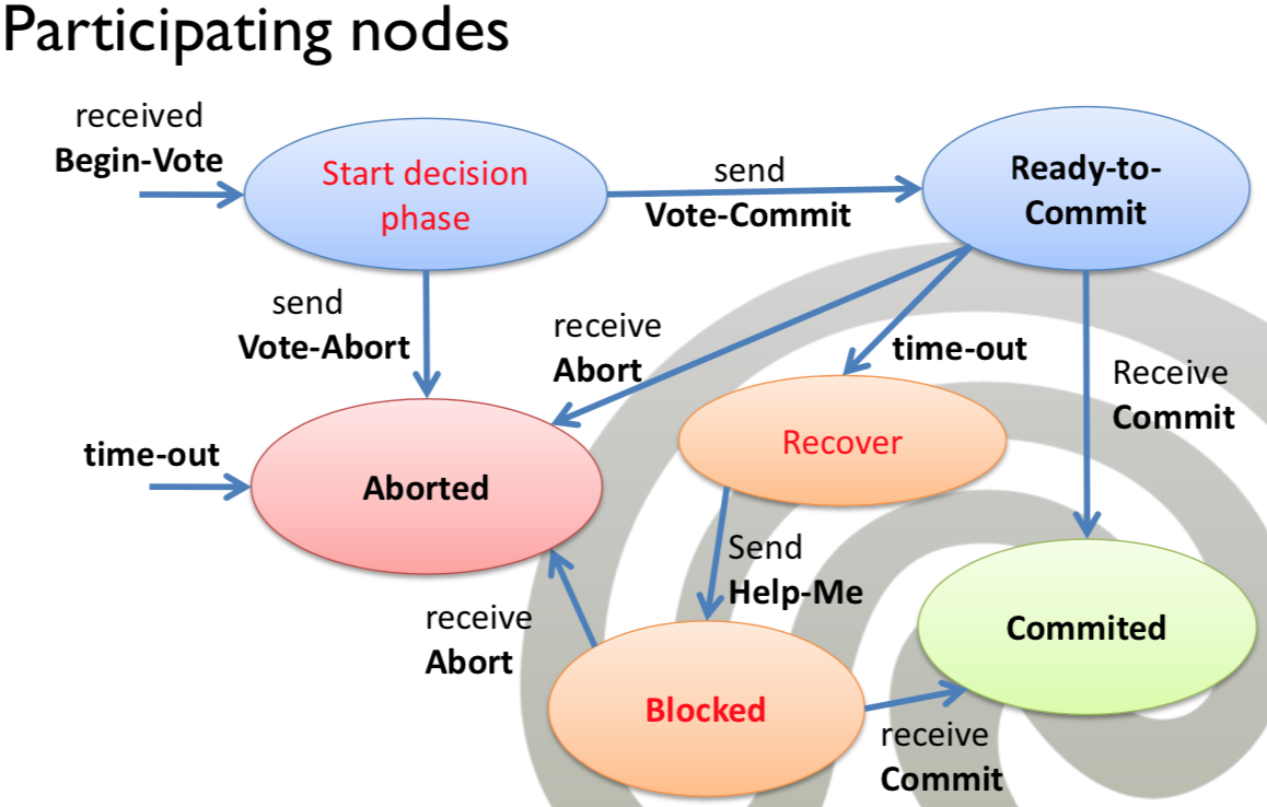
Distributed Two-phase locking

• Goal: Ensure consistency + isolation
• Central questions
  • How to handle locking in a distributed fashion?
  • How to handle locking with replication?
• Idea
  • Assume dependent sub-transactions
  • Generalize two-phase locking for distributed databases
  • Often used together with 2PC
• Parties
  • Central lock manager (LM)
  • Coordination manager (CM)
    • Manage transaction, get locks, distribute operations
  • Data processor (DP)
    • Execute operations
• Lock managers
  • Centralized D2PL
    • Single central lock manager
    • Bottleneck (unscalable, Single point of failure)
  • Primary copy D2PL
    • Multiple lock managers
    • Each responsible for certain partition
  • Distributed D2PL
    • Every node could be lock manager
    • Lock manager at each site
    • Useful for heavy replication (multiple network connections, load balanced)
    • Agreement with other lock managers
• Replication
  • Lock manager and transaction manager need replication information
  • Protocol for replication needed
  • Simple approach
    • Lock all copies of data item
    • If item is updated, CM must update all copies

Enterprise Applications

• Transaction may involve heterogeneous data sources
• Need federated transaction management (e.g., application server)
• Participating databases require interface: X/Open XA
• Example
  • Java Transaction API
  • X/Open XA
  • SAP HANA

X/Open XA

• Protocol for distributed transaction processing
• Each DBMS
  • Needs to support XA
  • Maintains integrity of wn data
• Uses D-2PL
  • Centralized transaction manager

SAP HANA

• Main-memory database
• Features
  • Main-memory + disk-based
  • Data structure optimized for main memory
  • Column store/row store/graph store
  • Efficient compression
  • ACID
  • OLTP + OLAP
  • Structured/unstructured data
  • Legacy/new applications
  • Massive parallelization
• Motivation
  • Decreasing memory cost
  • Increasing computing power
• Architecture
  • Languages: SQL, MDX, FOX
  • Engines: Relational Engine, Graph Engine, Text engine
  • Transaction manager
  • Persistency layer (logging, recovery, page management)
• Column store
  • Store rows as columns
  • Dictionary compression
    • Sort values ascending
    • Store index numbers in original order
  • Advantage
    • Faster-access
    • Better compression
    • Better parallel-processing
• Transaction management
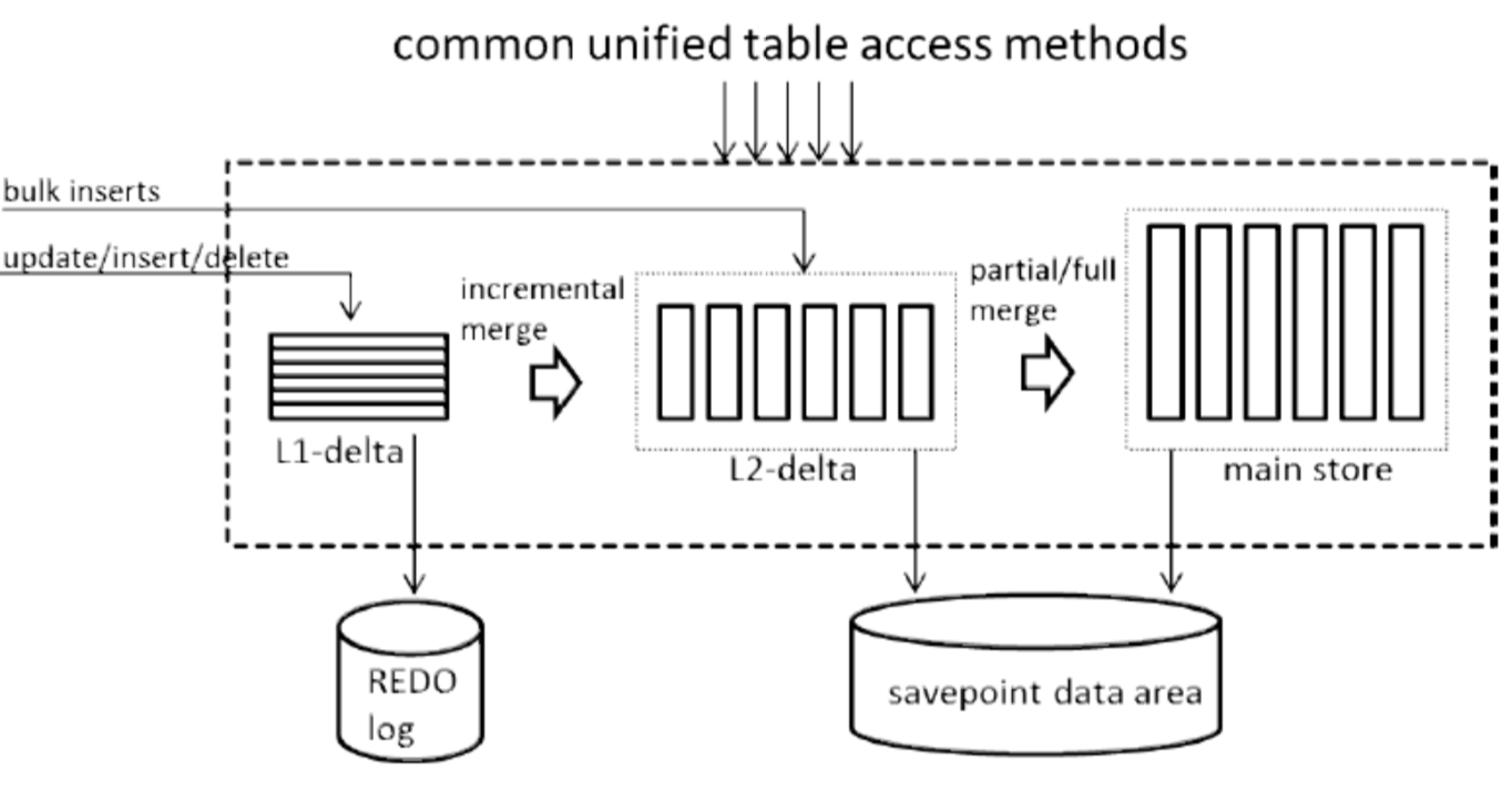
  • L1-delta: Update/insert/delete for REDO
  • L2-delta: Merge data
• Consistency
  • Consistent View Manager manages visibility of records per table
  • Table with transactions
    • TxID, status, CommitID
    • Transaction token acts as metadata
  • Multi-version concurrency control
    • Distributed snapshot isolation (Isolation)
    • Distributed locking (D-2PC)