Physical storage
Storage Media
Relevant media characteristics
- Metrics:
- Capacity
- Cost per capacity
- Random Access Time:
- Avg. time access random piece of data
- Transfer rate:
- Avg. amount of consecutive data transferred per time
- Volatile:
- Memory needs power to keep data
- Dynamic / static
- Access Modes:
- Random/sequential (only sequential order (tape))
- Write mode:
- Mutable storage: Read + write
- Write once read many (WORM)
- Media types:
- Online: Always on (Hard drive, main memory)
- Nearline: Compromise online/offline (e.g. tape robot library)
- Offline: Connect manually, tape basement
Storage hierarchy
- DMBS optimize data distribution among the levels
- Primary storage (Fast, expensive, usually volatile, limited capacity): Frequently used data / current work data (~100 ns)
- Secondary storage (Slower, large capacity, lower price): Main stored data (~10 ms)
- Tertiary storage (even slower, huge capacity, even lover price, usually offline): Backup / long term storage (> 1 s)
HDD
General
- current standard: cheap + persistent
- DBMS optimized for HD
- Fast access
- Often used data faster than rarely used data
- How does it work?
- directionally magnetization of ferromagnetic material
- Hard disk platters (base platter non-magnetic)
- Magnetic grains in platter for magnetic regions (1 Bit)
- Read head: Detect magnetization
- Write head: Change magnetization
Notable Technology advances
- Giant Magnetoresistance Effect (GMR)
- Efficient read heads
- Perpendicular recording
- allows 1000 Gb / inch^2
- Align magnetic field orthogonal to surface
- Magnetic grains instead of continuous material
- Neel spikes increase transition width (Unsure magnetic direction
- Grains have smaller transition width
Architecture
- Platter > Surface > Tracks > Sector
- Multiple double-sided platters
- Fixed on spindle
- Read and write head per surface
- Heads attached to arms
- No independent movement
- Platter side: Surface
- Surface divided in tracks
- Tracks with same diameter: Cylinder (efficient access)
- Track divided into sectors (equal capacity)
- Fixed angle sector (same number of tracks, changing density)
- Fixed data density (outer track more sectors)
- Adjacent sectors: clusters
Hard disk reliability
- Reasons:
- Contact cyles
- Spindle start-stop
- Power-on hours
- Unstable voltage
- Assumptions:
- Desktop usage: 2400 hours, 10000 motor starts, 25 °C
- Server usage: 8760 hours, 250 motors stars, 40 °C
- Non-recoverable read errors
- Corrupted sector
- Maximum contact cycles
- Maximum number allowed head contacts
- Mean Time Between Failure MTBF
- Time for disk population failing to 50 %
- Annualized Failure Rate AFR
- Probability of a failure per year (based on MTBF, operatingHours/MTBF)
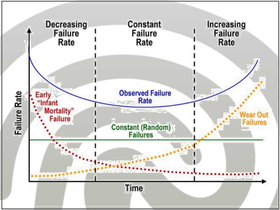
- Bathtub curve:
- Infant morality rate
- Wear out failure
- Random failure
Controller
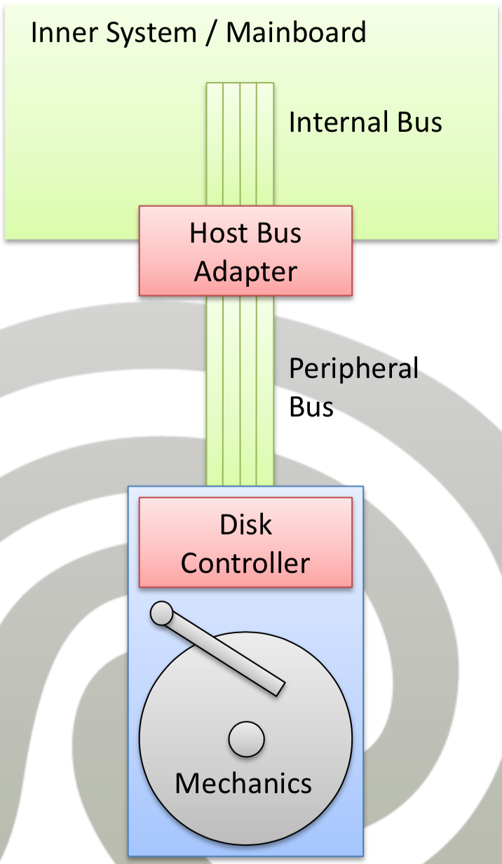
- Disk controller
- Low level access to disk
- Head positioning, error checking
- Connects disk to peripheral bus (IDE, SCSI, SATA)
- Abstracted (LBA) or unified interface
- Transfers content of whole blocks into buffer (primary storage)
- Block transfer time:
- Seek time + Latency (Rotational delay) + Block transfer time
- Host bus adapter (HBA):
- Bridge between peripheral bus and systems internal bus (PCI)
- Directly Attached storage (DAS)
- OS groups sectors to blocks
- Hardware address of block:
- Cylinder number, surface number, block number in tracks
- Controller maps hardware address to logical block address (LBA)
SSD
- microchips with data (non-volatile, no moving parts)
- Key components: Memory, controller
- Advantage:
- low access time + latency
- No moving parts -> schock resistant (MTBF 1,5 million h)
- Light
- Energy-efficient
- Disadvantages:
- Divided into blocks/pages
- Limited ability of being rewritten (100000 cycles per page)
Non-volatile memory
- Dynamic Random Access Memory (DRAM)
- Volatile
- Ultrafast access (< 10 microseconds)
- Sometimes internal battery
RAID
- Problem single HD:
- Limited capacity
- Limited speed
- Limited reliability
- Idea:
- Redundant array of independent disks
- Treat multiple hardware disks as a single logical disk
- Advantages:
- Increased capacity
- Parallel access
- Controlled redundancy
- Disks are virtualized
- Directly attached storage
Principles
- Mirroring
- Increase reliability by complete redundancy
- Idea: Mirror disks are exact copies of original disks
- Increase read speed, unchanged write speed
- Striping
- Improve performance by parallelism
- Idea: Distribute data among all disks
- BitLevel Striping
- Split bits of byte
- read/write increases
- no simultaneous access
- Good for few sequential large access
- BlockLevel Striping
- Distribute blocks
- Read/write of multiple blocks increases
- Good for large number of parallel accesses
- Error correction codes
- Increase reliability with computed redundancy
- Hamming codes
- Detect & repair 1 bit error within a set of n data bits with k parity bits
- \( N = 2^k - k - 1 \)
- Not really used for hard drives anymore
- Interleaved parity (Reed-Solomon Algorithm)
- repair 1 bit errors (error is known)
- Parity bit \( D_P = D_1 \oplus ... \oplus D_N \)
- \( D_1 = D_P \oplus ... \oplus D_N \)
Practice
- Mean Time To Repair (MTTR)
- MTTR = TimeToNotice + Rebuild Time
- Assumption: TimeToNotice = 0.5h
Levels
- RAID 0:
- Block-level-striping only
- \( MTBF / D \)
- RAID 1:
- Mirroring only
- \( MTBF^D / (D! * MTTR^{D-1}) \)
- RAID 2:
- Bit-Level-Striping (not used anymore)
- RAID 3:
- Byte-Level-Striping
- Interleaved parity, bottleneck
- RAID 4:
- as RAID 3
- Block-Level-Striping
- RAID 5:
- as RAID 4
- Parity is distributed
- RAID 6:
- as RAID 5
- Two independent parity blocks distributed
- RAID 1+0:
- Mirrored sets nested in a striped set
- High read/write speed
- increased reliability
- limited size
File Systems
- File System:
- Software for abstracting file operations on logical storage device
- Raw Devices:
- Bypass OS and filesystem (direct access on storage, efficient implementations)
NAS
- Idea: Abstracted file systems via network (software solution)
- NAS: Network Attached Storage
- Advantages:
- Easy setup
- Cheap infrastructure
- Sharing
- Easy for applications
- Disadvantages:
- Inefficient / slow
SAN
- Virtualized logical storage within a specialized network on block level (hardware solution)
- High-speed network for storage devices
- Specialized storage protocols
- Raw block level access
- Client has full control over logical disk
- Advantage:
- Very efficient
- Very flexible
- Good for disaster protection
- Disadvantage: Expensive
Indexing
Why Indexing?
- Problem: Efficiency of data access
- Depends on:
- Hardware used
- Data allocation on the disk
- Intelligent buffer management
- Access paths / indexing data
- DBA’s important task: Physical tuning
- Database in files (protected file system part)
- File partitioned into fixed length blocks (pages)
- Smallest unit transferred
- Size specified on DB creation (multiple of FS block size)
DBMS Blocks
- Hard disk sector abstracted by file system blocks
- File system blocks abstracted by DBMS blocks
- Overhead & Payload:
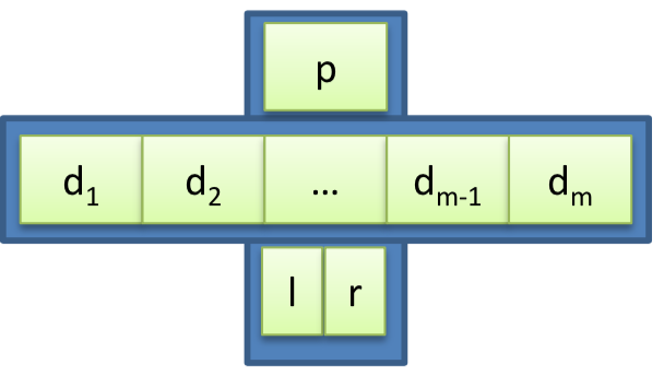
- Header (general blocks information, block address)
- Table directory (tables that have rows in this block)
- Row directory (information about rows in block, adresses, IDs)
- Row data
DBMS Buffer management
- Buffer manager: Hold copies of blocks
- Improvement: Optimized pre-fetching
- DB requests data record
- If block buffered, return memory address
- If block not buffered, allocate space, fetch block, return memory address
- Block replacement (different strategies)
- Modified block must be written to disk
- Modified block can’t be evicted, NEVER
- Block writing (depends on recovery strategy)
- Pinned block: cant be written
- Buffer replacement strategies
- Least recently used
- Toss immediate
- Expected reuse
Buffer replacement strategies
- Least recently used (LRU)
- replace oldest block
- Simple + effective
- Ignores semantics of data
- Toss immediate
- After DB processing a block, immediately replace
- E.g. block-nested loop join
- Expected reuse
- use statics about query frequencies
- Determine how useful a block is
- E.g. index blocks are accessed more often
Extents, Segments, Tablespace
- Extent
- logical collection of blocks (adjacent)
- Fixed size
- Segment
- Collection logically connected extents
- E.g. tables, indexes, rollbacks
- Tablespace
- logical storage space needed for data in table
- Grouping of multiple files
- Good practice: Tablespace for tables, tablespace for indexes
File organization
- Records of different relations -> different files
- Related records -> same block (minimize disk access)
- Multitable clustering: Records of different tables in same block (frequent joins)
- Record placement in file:
- Heap (place record anywhere)
- Sequential (store records sequentially, maybe indexed)
- Hashing (hash function determines block of file)
- Write records (Goal: retrieving with minimal disk access)
- Fixed length records
- Variable length records
- Record organization in blocks:
- Spanned (pointers divide records)
- Unspanned (fill block with complete records)
Fixed length records
- Easy to implement
- Problem: Block size must be multiple of record length
- Problem: Deleting a record
- Mark as deleted: Slow reading
- Replace it: Sequence changed
- Move other items: Low efficiency
- Pointer list: Wastes space
Variable length records
- Storage space efficient
- Necessary for multi-table files or records with variable length attributes
- Problem: Where does a record end?
- End-of-record symbols (Record update?)
- Store record length (Record update?)
- Slotted page structure: Block header has number of entries, end of free space
Non-Standard blocks
- Large objects:
- Binary large objects (BLOBS)
- Character large objects (CLOBS)
- no interpretation in the database
- Store in continuous byte sequence
Indexing
- Goal: Locate records in DB quickly
- Ordered by indexing field (search key)
- Index file has index entries (search key: record location)
- Types of queries
- Exact match (certain value)
- Range queries (certain value range)
- Types of indexes
- Ordered indexes (Search keys stored in order): Single-level ordered indexes, Multi-level ordered indexes
- Hash indexes (Search keys distributed uniformly across blocks using hash function)
- Index every attribute? No! Updates slow (multi-level index: update every level)
Single-Level Ordered Indexes
- Index file:
- Dense index: Index all items
- Sparse index: Index only selected items
- Small: Binary search fewer block access than data file
- Index sizes:
- Primary index: Number of blocks
- Clustering index: Number of distinct search keys
- Secondary index: Up to number of records in table
Primary index
- order data by unique attribute
- Index record contains pointer to block address
- Possibility to save entries
- Index entry per block (block anchor)
- Problem: Index doesn’t show whether a record exists
- Advantages
- Number of block needed is small compared to data (sparse, index entries smaller)
- Often kept in buffer
- Disadvantages
- Insertions/deletions need to move data (shifting)
Clustering index
- Order data by non-unique indexing field
- One entry in index per distinct value of indexing field
- Search key linked to block address
- Sparse index
- Index does show whether a block exists
- Problem: Insertion/deletion (often more than one block is needed, linked by pointer, not necessarily adjacent)
- Structurally similar to hash index
Secondary index
- point to location with non-ordering attribute
- Not affecting storage order
- Usually dense
- Records with adjacent values are not adjacent on disk
- Unique indexing field: Index all records
- Non-unique indexing field:
- Dense index with duplicate search keys
- Variable length index entries with list of pointers
- Indirection: Point to block with pointers (used in practice)
Characteristics
- Characteristics of secondary indexes
- Speed up retrieval (otherwise table scan)
- More search time (because dense)
- Provide logical ordering (maybe inefficient because not ordered physically)
- Secondary index for range queries:
- Problem: Same block unnecessarily accessed multiple times
- Remember: Blocks in main memory cheap, fetching expensive
Multi-Level Ordered Indexes
- Possible Problem:
- Primary index does not fit in main memory
- Bad lookup efficiency
- Solution: Multi-level index
- Treat primary index on disk as file, construct sparse index on it
- Outer index: Sparse index of primary index
- Inner index: Primary index
- Outer index too large, add new level
- Efficiency: \( \log_{fanout} N \)
- Can be applied to primary, secondary and clustering index (distinct values)
- Structures for multi-level indexing: B-tree, B*-tree, R-tree
Hash Indexes
- Fixed-size index space \( [0, M] \) with \( M+1 \) buckets
- Buckets contain links to data
- Single link internal hashing (data to bucket, in-memory)
- Multiple links external hashing (bucket to data, hard disk)
- Hash function
- Uniform distribution
- Surjective (use full range)
- Deterministic
- Simple
- Fast
- Idea: Convert search key to number, hash it, store block anchor in bucket
Problems
- Problem: Collision
- Hash function not injective (Overflow lists for full blocks)
- Worst case: \( O(n) \)
- Problem: Static address range
- Addressable range fixed to \( [0, M] \)
- Load factor too high, many collisions
- Solutions
- Rehashing: Create larger hash map (expensive)
- Extendible hashing: Dynamic directory to double and half number of buckets
- Linear hashing: Split bucket, rehash with additional hash function
Extendible hashing
- Represent values as bit string
- Create directory with global depth \( d \) (\( 2^d \) entries)
- First d bits of bit string determine bucket
- Local depth determines how many bits are used for this bucket
- Insert: Bucket overfilled, split bucket with local depth + 1
- Dynamically split/union buckets as database grows/shrinks
- If bucket full and local depth lower than global depth: split bucket, increase local depth
- If bucket full and local depth equally global depth: Increase global depth, double directory size
- Efficiency
- Overhead can be large
- Can perform \( O(1) \)
- Overflow lists: Small management overhead, decrease performance to \( O(n) \)
- Rehashing: Expensive for each stage
- Extendible hashing: Smaller overhead, suitable external storage hashing
Physical Tuning
- Tools: Snapshot monitors, event monitors
- Usually trial and error
- Measure metrics
- Adjust something (indexes, tablespaces)
- Measure again
- Database types
- OLTP: Small concurrent read/write queries
- Warehouse (OLAP): Large complex queries for retrieving
Snapshot monitor
- Monitor collects cumulative statistics
- Internal counters (global/session level)
- Point-in-time information: Locking, Bufferpools, sorts, tablespaces, Unit of Work, Dynamic SQL
- Continuous overhead is 3%-5% (no IO, all RAM)
- Useful metrics
- Bufferpool hit ratio
- Sort overflow/problems
- Effectiveness of prefetch
- Need for indexing
- Transaction logging issues
- Single queries/application resource domination
Event monitor
- Collect information regarding events/chained events
- Explicit creation + activation in DBMS
- Tasks
- Identify/rank most frequently SQL
- Track sequence of statements leading to a deadlock
- Connections to database
- View time of sub-operations (sort time)
Physical Tuning Metrics
- Average Result Set Size (ARSS)
- \( ARSS = \frac{RowsSelected}{NumSelectQueries} \)
- \( ARSS <= 10 \) for OLTP
- Index Read Efficiency (IREF)
- \( IREF = \frac{RowsRead}{RowsReturned} \)
- Should be lower 10 for OLTP
- Synchronous Read Percentage (SRP)
- DMBS reads just the index file for required data (good)
- Asynchronous: DBMS prefetches and scans for data
- Average Rows Read per DB Transaction per Table (TBRRTX)
- \( TBRRTX = \frac{rowsRead}{attemptedCommits + attemptedRollbacks} \)
- Average Read Time (ART)
- Average time per read
- \( ART = \frac{ReadTime}{NumDataRead + NumIndexRead} \)
- What to do? Adjust size of table space containers, distribute contains across disk
Trees
Motivation Trees
- indexes need suitable data structure (ordered for efficient look-ups)
- Important: Indexes in separate database file
- Search within index: Bisection search possible, spans several blocks
- Issues: Insertion (shift all indexes), Deletion (Mark as deleted)
Binary Tree
- Rooted, directed trees
- Each node has node, one or two children
- Each node (except root) has one parent
- Naming:
- Leaf node: node without children
- Depth of node: Length of path from root to node
- Height of tree: Maximum node depth
- Ancestor/descendant: Path between nodes exists
- Size of node: Number of descendants including itself
- Subtree of node: All descendents including itself
Binary Tree Types
- Full/proper binary tree:
- Each node has either zero or two children
- Perfect binary tree:
- All leaf nodes same depth
- Contains \( 2^h \) nodes
- Height-balanced binary tree:
- depth of all leafs differ by 1
- Contains between \( 2^{h-1} \) and \( 2^h \) nodes
- Degenerated binary tree:
- Each node has either zero/one child
- Behaves like linked list O(n)
Binary Search Tree
- Binary tree
- Each node has unique value
- Total order on values (left subtree smaller, right subtree larger)
- Simple, dynamic data structure
- Inefficient for degenerated trees
- Issues:
- Good for internal memory, not disk
- Nodes must be stored linearly (in blocks)
- Worst case: read all nodes during search (expensive)
- Inserting / Creation
- Insert values incrementally
- First value is root
- Order important
- Efficiency: \( O(n) \) worst case, \( O(\log n \)) average case
BST: Search
- Start with root
- Recursion
- If node value = v: Return node
- If node = leaf: Not found
- If v < node value: search left subtree
- If v > node value: search right subtree
- Complexity: \( O(\log n) \)
- Worst case: \( O(n) \) (degenerated)
BST: Traversal
- Access all nodes of tree
- Pre-order: visit node, traverse left, traverse right
- In-Order (sorted): traverse left, visit node, traverse right
- Post-order: Traverse left, traverse right, visit node
BST: Deleting
- Locate node
- If node leaf: Delete it
- If node has one child: Delete node, attach child to parent
- If node has two children
- Replace w/ in-order successor (left-most child right subtree)
- Replace w/ in-order predecessor (right-most child left subtree)
- Complexity: \( O(\log n) \)
- Worst case: \( O(n) \)
Self-balancing BSTs
- Observation:
- BST efficient if perfect or balanced
- Idea:
- Continuously optimize tree structure (keep balanced)
- Popular:
- AVL-Tree
- Red-Black-Tree
- Splay-Tree
- Scapegoat-Tree
Global rebuild: Lazy deletion
- Basic concept for deletion
- Lazy deletion
- Start with balanced tree
- Mark node as deleted
- Rebuild condition: Rebuild whole tree without deleted nodes
- Search efficiency
- \( n \) number of unmarked nodes
- Tree has max \( 2n \) nodes (balanced)
- Number of accesses usually increased by 1
- Delete efficiency
- Global rebuild in \( O(n) \), amortized \( O(1) \)
- Average: \( O(\log n) \)
- Worst case: \( O(n) \)
Global rebuild: Direct deletion
- Direct deletion with rebuild
- delete nodes as normal binary tree
- Increment deletion counter
- Rebuild tree if counter has specific value
- Complexity similar as with lazy deletion
Local balancing (Subtree balancing)
- Basic concept for Insertion/deletion
- start with balanced tree
- Insert/delete nodes normally (subtree too balanced, locally balance)
- Unbalanced condition:
- \( |h(left(v)) - h(right(v))| > a \) (a ist konstant)
- Alternative unbalanced condition:
- \( h(v) > a * log2 |v| \)
- After inserting node, walk back, update statistics
- Local balancing:
- Rebuild subtree
- Expensive
- \( O(n) \) worst case, \( O(\log n) \) average
- Can optimize physical storage
- Suited for disk-based tree
- Rotating
- Move pointers (very efficient)
- \( O(1) \)
- No physical storage change
- Suited for memory-based trees
- Types: Simple (left, right), Double (Rollercoaster, Zig-Zag)
Block Search Tree
- Node complete DB block
- Store q pointers (link to subtree)
- Store \( q-1 \) key entries (index entry)
- Only one disk access per tree height
- Optimized for disk storage
- Average case \( O(\log_{fanout} n) \)
- Inefficient for degenerated trees
- Similar to binary search trees
Block Search Tree: Search
- Recursive
- Start root
- Bisection search in current node
- If key found: Return it
- If key not found:
- If pointer between two values: Follow link and recurse
- Else: Key not found
Block Search Tree: Insert
- Start with root
- Bisection search in current node
- Key found: Abort
- Key not found
- Pointer between two values: Follow pointer and recurse
- No pointer found
- Space left in key: Insert key, restore order
- No space left: create empty node, insert key to node, link to current node
Block Search Tree: Delete
- Start root
- Locate k
- k in leaf node: Delete k from node, restore order (node empty: delete node)
- k in internal node
- No or only one adjacent pointer of k used: Delete k, restore order
- k is separator between two used pointers
- Space in both subnodes sufficient: Union nodes, delete k, restore order
- Space not sufficient: Replace k with new separator (largest from left or smallest from right)
B-Tree
- Ideas
- Search within DB block efficient (blocks as tree nodes, search in-memory)
- Read block from disk expensive (reduce reads, data in leaf nodes)
- Minimize tree height (increase fan-out factor)
- Properties
- used for disk-based indexing
- Key may be non-unique
- Tree self-balancing (no degeneration)
- \( O(\log n) \) for all operations (\( \log_{fanout}((n+1)/2) \))
- B-tree node:
- Contains key value and data pointer
- Node pointer for left/right subside
- Changes to Block Search tree:
- Guaranteed fill degree (Node between L and U links, \( 2L=U \))
- Self-balancing
- During insertion: Split node if more than \( U-2 \) keys
- During deletion: Union nodes if less than L keys
- Node created/deleted use local rebalancing
B-Tree: Insert
- Insertion starts at leaf node
- If |leaf node| < U:
- Insert + restore order
- If |leaf node| = U:
- Perform node split
- Node split operation:
- Choose new separator key
- Median from leaf node elements and the new
- Add separation to parent (another split possible)
- Lower bound does not apply to root
B-Tree: Delete
- Issues:
- Deleting problematic (decrease unter minimum elements possible)
- Element to be deleted could be separator for children
- Deletion from child (can cascade to root)
- Delete key, check for rebalancing
- Deletion from inner node (can cascade to leaf)
- Case 1) Both two children at minimum
- Create one single node (joining)
- Case 2) One of the children has more than minimum
- Choose new separator for key to delete (in-order predecessor or successor)
- Case 1) Both two children at minimum
- Rebalancing after deletion / Stealing
- If leaf node is under minimum size, redistribute elements from siblings to bring all children back to minimum
- If all children are at minimum size, parent node must provide an element
B-Tree: Rebalancing
- Rebalancing strategy
- Goal: Find sibling with more elements than minimum
- Steps:
- Choose new separator (in-order predecessor or successor, order is not important)
- Move new separator to parent
- Put old parent separator to deficient node
- Special case: Both siblings at minimum
- Union nodes from one sibling, the deficient node and the parent separator
- Remove old parent separator and add hang in new node
- This can cascade to the root
B*-Tree
- Constrained B-Tree
- All non-root nodes need to be filled 2/3
- Better than B-Tree but lost importance
- File systems: HFS, Raiser 4
B+-Tree
- Optimized B-Tree
- Improved traversal performance
- Improved search efficiency
- Improved memory efficiency
- Uses different nodes
- Internal: Only unique key and no data pointers, for search guidance
- Leaf: Keys with data pointers, inter-linked (good for range queries)
- Super index structure for disk-based databases
IMDB
- Observation: Hard disk major bottleneck
- Idea: Store all data in memory
- Solutions:
- DBMS with huge buffer
- In-memory database system
- VoltDB: Operational database
- Advantages: No locking, no logging, ACID compliant, fast
- Disadvantages: Difficult and expensive setup, several clusters
- Problem durability:
- Checkpoints (only partial durability)
- Transaction logging
- NVRAM (SRAM with battery)
IMDB Indexing
- B-Tree: Shallow + bushy (unnecessary for RAM)
- Hash index: Very fast, but storage overhead
- T-Tree (main memory cheap access, Blend AVL and B)
- Self-balancing tree (like AVL)
- Nodes contain only links
- Node links m data records (ordered)
- Node links to parent
- Node links to left and right
- Fill degree: \( c_{min} - c_{max} <= 2 \)
- Chained bucket hashing
- No range queries
- Storage overhead
CST-Tree
- CPU Cache speed increased
- Cache misses in T-Tree
- Big part of CPU data not used
- Cache-sensitive T-Tree
- Usage of cached data (binary search)
- Node size equals cache line
- Search performance improved by 65 % to classical T-Tree