Query optimization

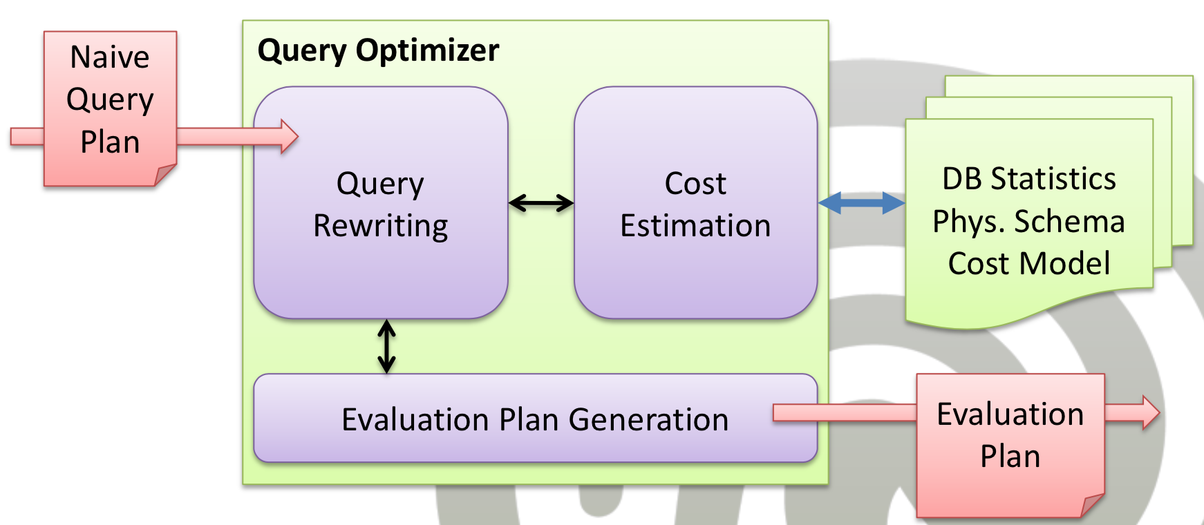
Query Optimizer

• Heart of Query Processor
• Tasks:
  • Translate query into RA (naive query plan, really?)
  • Transform into efficient plan (physical operators, operator sequence + grouping)
  • Keep semantics
  • Annotate plan
  • Give to evaluation engine
• Approaches
  • Bottom-up: Optimize queries, generalize algorithms
  • Top-down: Algorithms for classes of queries (common)
• Optimization (hybrid common)
  • Heuristics: Works for most queries
  • Cost-based: Good for specific queries

Pipelining

• Idea: Pipeline results between operators
  • e.g. pipeline join into selection, on-the-fly selection
• Advantage:
  • No temporary tables
  • No expensive writing/reading
• How does it work?
  • Tuples passed over operators (operation has buffer)
  • Execution:
    • Demand-driven (top-down, pull)
    • Producer-driven (bottom-up, push)
• Demand-driven
  • Important: Coordinate execution
  • Use Iterator interface (open, getNext, close) to hide implementation details
  • Restriction
    • Works for selection, projection, index nested loop join
    • Works not for sorting, hash join, merge join
    • Materialization can be more efficient

Algebraic query rewriting

• Idea: Find best plan before executing query
• Rewriting: RA equivalences (use transformation rules, result never changed)
• Static plans:
  • Best plan known a-priori for query class
  • Access paths, operator sequence saved
• Dynamic plans:
  • Best plan must be found at run-time
  • e.g. heterogenous query behavior

Selection

• Cascading: –TODO: Formula–
• Commutativity: –TODO: Formula–

Projection

• Cascading: –TODO: Formula–
• Commutativity PI with SIGMA: (selection work on projection)

Joins

• Commutativity: –TODO: Formula–
• Associativity: –TODO: Formula–
• Join construction: –TODO: Formula–
• Commutativity SIGMA with JOIN: –TODO: Formula–
• Commutativity PI with JOIN: –TODO: Formula–

Set operators

• Commutativity UNION / INTERSECTION: –TODO: Formula–
• Associativity UNION / INTERSECTION: –TODO: Formula–
• Commutativity SIGMA with SETS: –TODO: Formula–
• Commutativity PI with SETS: –TODO: Formula–

Cost-based optimization

• Problem: No always optimal plan exists
  • Efficiency depends on instance, implementation, access paths and indexes, etc.
• Idea: Assign average costs to operators -> estimate total cost (profit function)
• Usage:
  • Database statistics
  • Result sizes
  • Block accesses

Database Statistics

• Statistics reveal bottlenecks
• Focus
  • Block accesses: assumes I/O-bound bottleneck (common, index-reading ignored)
  • CPU statistics: assumes CPU-bound bottleneck (IMDBs)
• Annotate operators:
  • Cost of performing (input size, indexes, I/O, processing, pipelining, materialization)
  • Size of result (expected input for parent, distinguish sorted/unsorted)
• Estimation parameters (based on system catalog)
  • Database buffer size
  • Cardinality of input base relations (number of records, number distinct domain values)
  • Relation size (pages on disk)
  • Available access paths (index cardinalities: #keys, #pages, height, ranges)

Estimation Result Sizes

• Goal: Keep intermediate results small
• Max. size: Product of relation cardinalities
• Selections: Selectivity, reduction factors
• Projection: No effect
• Assumption: All reduction statistical independent
• –TODO: Formula 5.36–
• Estimate reduction factor
  • Column = value
  • Column = Column
  • Column <,> value
  • Column IN {List}

Estimation Reduction Factor (Equality selection)

• COLUMN = VALUE
  • No index: Use distinct values + histograms (or \( rf = 0.1 \))
  • Index: \( rf = 1 / \#keys(I) \)
• COLUMN = COLUMN
  • Index on both: \( rf = 1 / _max(\#keys(I_1), \#keys(I_2)) \) (Assumption: smaller I SUBSET larger I)
  • Index on one: \( 1 / \#keys(I) \)
  • No index: distinct values

Estimation Reduction Factor (Comparison + List)

• COLUMN <,> VALUE
  • Index: \( rf = (high(I) - value) / (high(I) - low(I)) \)
  • No index / no arithmetic type: \( rf = 0.5 \)(Assumption: value in middle of domain)
  • Range queries: Disjunction of both conditions
• Column IN {list}
  • Index: \( rf = \#listvalues * (1 / \#keys(I)) \)(usually at most 0.5)
  • Column IN (subquery)
  • rf = estimated subquery result / number of distinct values in column outer relation

Estimation Block Accesses (Equality selection)

• COLUMN = VALUE
  • Assumption: Uniform value distribution, available index
  • Depends on type of index + result size
  • Primary index: #blocks = 1
  • Cluster index: #blocks = #result size / (#recordsR / #blocksR)
  • Secondary index: #blocks = #result size
  • No index: #blocks = #blocks
• COLUMN = COLUMN
  • Depends on selectivity of join (-> Join order optimization)
  • Worst case: Cartesian product (#blocks = #blocksR * #recordsS

Estimation Block Accesses (Range selection)

• COLUMN <,> VALUE
  • Assumption: Uniform value distribution, available index
  • Depends on type of index + result size
  • Primary/cluster index: #blocks = #blocksR / 2
  • Secondary index: #blocks = #recordsR / 2
  • No index: #blocks = #blocksR

Access Path Decision

• Problem: Multiple indexes available
• Idea: Choose right access -> low I/O bound efficiency
• Selectivity of access path: #pagesFetched / #allPages

Single-level index

• Implementation: Predicate splitting
• Per condition: Compute least expensive form of evaluation
• Start with least expensive method
• Apply all other conditions
• Result: Suboptimal but sufficient

Multi-level index

• Useful if conditions are index with secondary index
  • Set intersection of block- or record-IDs
  • Order result pointer set by block-IDs -> efficient access
  • Apply non-indexed selection afterwards

Sorted-index

• Useful if tree index exists and traversable in specific order
• e.g. GROUP BY / aggregations
• Apply selection on-the-fly
• Good for cluster indexes

Index-only

• Rarely possible, very efficient
• Requirement: All attributes are in dense index
• Apply selection directly on index entry

SQL EXPLAIN

• Show operation execution order
• Collect metrics for each operation
• Allows bottleneck analysis + manual query optimization
• EXPLAIN PLAN SET queryno= FOR

Query Plan generation

• Naive:
  1. Apply transformations -> generate all possible plans
  2. Assign costs
  3. Choose least expensive plan
• Problem: Prohibitively expensive
• Idea: Don’t search for best plan, but avoid bad plans (Local minima are ok)

Heuristic optimization

• Goal: Alter tree to lower costs (use heuristics)
• Principle: Improve operator tree step by step
• Common assumption: Keep intermediate result small (less work, better buffer utilization)
• Optimization heuristics
• not always equally effective (query profile, statistics)
• „magic“ (DBMS’ unique selling point)
• Query Optimizer decides about heuristic

Simple heuristics

• Most important heuristics:
• Select as early as possible
• Project as early as possible
• Avoid cartesian product (or as late as possible)
• Use pipelining for adjacent unary operators
• Result: Vastly improved operator tree

Simple heuristics (Selections)

• Early selection => small intermediate result
• Advantage: Better DB buffer utilization / faster processing (less records)
• Break selections (where statement CNF)
• Push selections down
• Caution: Joins (dont push into indexed join => don’t destroy index)

Simple heuristics (Projections)

• Early projection => Minimize record size
• Shorter records => more records per block
• Push projections down (caution: selections)

Simple heuristics (Cart. products)

• Problem: Cartesian product => expensive
• Solution: Use native joins (more efficient)
• Force joins (merge selection and Cartesian product)

Hill climbing

• Greedy strategy (apply simple heuristics)
• Input: canonical query plan
• Output: Improved query plan
• Break selections
• Push selections down (as far as possible)
• Break, Eliminate, Push, Introduce projection
• Collect seletions/projections (OP1 - SIGMA - PI)
• Introduce joins (merge selections and cartesian product)
• Prepare pipelining

Complex heuristics

• Sophisticated heuristics
• Special operations
• View merging
• Eliminate common sub-expressions
• Replace uncorrelated sub-queries by joins (Flattening)
• Sort elimination
• Dynamic filters
• Exploit integrity constraints (semantic knowledge)
• Selectivity reordering
• Problem: Can fail (no perfect optimizer)
• Trade-Off: Sub-optimal query execution vs. optimization time
• Solution: Optimization hints

CH: Special operations

• Use special algorithms for specific subtrees / operation patterns
• Example: Non-standard join (Semi-join, anti-join, nest-join)

CH: View merging

• Problem: View computation at query time (expensive)
• Solution: Replace view with view definition (if not required)
• Advantage: More freedom to optimize operator tree => better plan

CH: Common sub-expressions

• Different operations need same input (multiple evaluations)
• Solution
• Logical rewriting (DeMorgan’s law)
• Materialization

CH: Sub-Query flattening

• Subqueries are optimized independently
• Problem: Plan can be suboptimal (e.g. selection not applied early)
• Problem: Result not processed after retrieval (but duplicate elimination could be efficient)
• Solution: Rewrite subquery as join (or semi join for duplicate removing)

CH: Sort elimination

• Problem: Most resource intensive operation
• Intermediate result already sorted
• Sort-merge join
• Retrieval in-order (e.g. PK)
• Unique-constraints
• Solution: Don’t sort again

CH: Dynamic filters

• Situation: Joins/Views computed completely but are later restricted
• Solution: Create dynamic restriction (filters), push into operator tree
• E.g. create semi-join with parents to only select „John“
• Result: Small intermediate results
• —Image 43—

CH: Semantic knowledge

• Use semantic knowledge for optimization
• Use dependencies/integrity constraints
• Strong technique but requires manual interaction
• e.g. replace conditions (higher selectivity), semantic transformations (different access paths)

CH: Selectivity reordering

• Apply operator with lowest selectivity first (smallest size, fewest records)
• Use statistics (difficult) / guessing
• Important: Join order optimization
• Correlation of columns: Expensive, exponential combinations
• Transient data (intermediate results): No statistics available
• Dynamic sampling (Oracle 10g): Gather additional statistics during optimization
• Gather sample set of tables
• Test statistical connections on the fly

Optimizer hints

• DB Administrator gives optimization hint (what-if-analysis)
• Alternative access path (provide fallback)
• Modify PLAN_TABLE
• When to use?
• Temporary fix for bad plans
• Access path regresses (version update, statistics update) => Revert plan
• Optimizer unable to find good plan (additional statistics required, complex query)
• Manual access path (prevent optimizer from changing plan)
• Excessive optimization time (complex join, memory/CPU consumption)

Join Trees

• Join commutative/associative => eval. in every oder
• Result: Join tree (different shapes, different assignments)
• Different trees => different evaluation costs
• Number of shapes (Catalan number): —Formula—
• Number of assignments per shape: n!
• Number of assignments: T(n) * n!

Join Order Optimization

• Find most efficient join tree / join implementation: NP-hard
• Task: Find good plan in sensible time
• Naming: Left: Build relation / Right: Probe relation
• Desirable join cases:
• Block-nested loop join (smaller rel. in-memory, inner loop)
• Single-pass join (best case)
• Build rel. fits into main memory
• Index-nested loop join (index on probe, inner loop, small build)
• Optimizer choices:
• Consider all trees: Impossible
• Consider class of tree: Select shape
• Use heuristics
• Find best solution: Dynamic programming / Branch and bound
• Approximation: Greedy strategies, randomized strategies (II/SA), genetic algorithms

Join Metrics

• Goal: Evaluation join costs
• Estimated result size
• same for all assignments
• Worst: Cartesian product
• Estimated cost
• Cost for performing join
• Consider CPU, I/O, buffer statistics, join algorithm

Join Metrics (Size)

• |R JOINc S| = |R| * |S| * rf
• 1. Theta-Join: rf = 0.5
• 1. Natural/equi-join (R.A = S.A)
• 2.1) R and S disjoint: rf = 0
• 2.2) Keys and foreign keys
• A is key of S / foreign key of R: rf = 1 / #dv(R, A) = 1/|S|
• A is key of R / foreign key of S: rf = 1 / #dv(S, A) = 1/|R|
• Keys unknown: rf = 1 / max(#dv(R, A), #dv(S, A))
• 2.3) R and S same values: rf = 1
• Result size
• Single equality condition: rf = 1 / max(#dv(R, A), #dv(S, A))
• Multiple equality conditions: Multiply reduction factors
• Multiple relations: Cascade formula (order irrelevant)
• Improve accuracy:
• Histograms
• Dynamic sampling
• Simulating common queries
• Incorporating previous query results
• More statistics are expensive w/ high change rate

Join Metrics (Execution cost)

• Goal: Minimize execution cost
• Cost metrics
• Size of intermediate results
• Block accesses
• Size of intermediate results
• costs(R JOIN S) = 0
• costs(R JOIN S JOIN T) = |R JOIN S|
• Ignores: Real I/O, memory, CPU, Join algorithm

Join Metrics (Access cost)

• Problem: Major bottleneck (depends on join algorithm)
• Costs writing result: |R JOIN S| / #blockingFactor
• Block-nested loop join
• Cost = bR * (1 + bS) + resultCost
• Index-nested loop join
• Cost = bR + (|R| * (Cix + 1)) + resultCost
• Index retrieval cost Cix
• In-memory index = 0
• Cluster index: Cost = indexAccessCost + SSIGMA / blockingFactor
• Secondary index: Cost = SSIGMA
• Hash index: Cost >= 1 (depends on hash size/collision)
• Sort-Merge-Join
• Cost = bR + bS + sortingCost + resultCost

Left-deep Join Trees

• Simple heuristic: Use left-deep join trees (only one tree shape)
• Advantage:
• Decrease build relation (good performance, good buffer usage)
• Pipeline results into next (no temp. table, but: not for sort-merge-join)
• Number of trees smaller (assignments, n!)
• Disadvantages
• Impractical for > 15 joins
• No parallel execution (dependencies)

Dynamic Programming

• Idea: Break problem into sub-problem / Memorize best solution
• Cost table
• Store lowest costs for joins (remember good solutions)
• Columns: Relation subset, estimated result size, estimated lowest cost, expression
• But: Uses buffer space
• Claim: Table always contains join expressions with lowest cost for gives relation subsets
• Guarantees best join order
• Exponential effort 2^n (10-15 joins)
• Space / memory consumption

Dynamic Programming (Induction)

• For each single relation subset: One row (cost = 0, size = |R|)
• For each relation subset size two
• One row (cost=0)
• Use heuristic to choose ordering (smaller to left)
• Induction:
• One table row per set
• Estimate size and costs (use cheapest subset)
• Find cheapest expression (size+cost)
• Left-deep tree: Add new relation to right
• Arbitrary shape: Add smallest to left, consider all partitions

Greedy Strategy

• Result not optimal but sufficient
• Goal: Quickly construct left-deep tree
• Algorithm
• Start with join pair with lowest cost (smaller relation to left)
• Incrementally add relation (the one with cheapest cost, attach to right, use distinct values)
• Drawback: Only heuristic (will not find optimal solution)

Randomized Algorithms

• Light-weight algorithm (low memory, can stop after specific time, usually finds good solution)
• Good: Solution space not enumerable (better than heuristics)
• Idea
• Solutions are points in space
• Connections (moves): Transform solutions
• Typical algorithms
• Iterative improvement (short optimization time)
• Simulated annealing (good solutions)

Randomized Algorithms (Typical moves)

• Typical moves (left-deep)
• Swap: Exchange position of two elements
• 3-Cycle: Rotate the arbitrary positions
• Typical moves (bushy tree)
• Commutativity
• Associativity
• Left join exchange
• Right join exchange

Iterative Improvement

• Problem with hill climbing: Too expensive (check all solutions)
• Start at random point
• Apply random move
• Check solution
• Less costly: Repeat
• More expensive: Undo operation, repeat (no better move found -> quit)
• Result: Random walk, local optimum
• Constant improvement
• quite efficient
• can’t leave local minima

Simulated Annealing

• Simulate natural annealing (first heating, slowly cooling)
• Start with random tree (hight temperature)
• Apply random move
• Proceed if less expensive or with probability P —Slide 57—
• Reduce temperature
• Problem: Parameterization (starting T, reduction, stopping condition)
• Two-phase-version (often used)
• Iterative improvement for several solutions
• Use least expensive result for sim.ann. (can start with lower T)

Randomized Trees

• Join Tree Generation
• Generate shape
• Generate relation assignment
• Cases:
• Generate Deep-Left tree
• Generate arbitrary shape

Randomized Trees (Deep-left)

• Task: Find random permutation of relations (quickly)
• Ranking/unranking
• Ranking: f:S->[0,n[
• Unranking: f:[0,n[->S
• Efficient unranking:
• Elements: [R1,…Rn]
• Algorithm: —Slide 63—

Randomized Trees (arbitrary shape)

• Generate code word: Dyck word
• Bijection Dyck word - binary tree
• Words of balanced number of characters
• Encoding Binary Tree
• Traverse tree pre-order (visit, left, right)
• Skip last leaf node
• Inner node: (/1, leaf node: )/0
• Mapping to Triangle
• Number of paths: Catalan number
• Unranking (use triangle grid)
• Integer to Dyck word
• n+1 relations (leafs) => Dyck word length 2n
• Ballot number p(i,j): Number of possible paths from (0,0) to (i,j)
• Use q(i,j): Number possible paths from (i,j) to (2n,0)

Randomized Trees (arbitrary shape, algorithm)

• ???