Datalog
Deductive Database
- Goal: Implement a deductive system
- Logic is the basic building block of a knowledge base
- Requirements:
- KB should be storage efficient
- KB should be easily extensible
- Deductive databases implement these goals
- Approaches:
- Relational Database
- Deductive Database
Example
- Store family trees with genetic predispositions
- e.g., Disease X is possible if genes \( G_1 \) and \( G_2 \) are inherited by parents
- Naive storage:
- Relational database
- \( R(name, parent, G_1, G_2) \)
- Problem:
- Ancestors are not directly stored
- Many self-joins would be required
- Very inefficient
- Idea: Change of the schema
- Store all ancestors directly
- Problem: Results in exponential storage costs
- Types of knowledge:
- Static/provided knowledge
- Derived/rule knowledge
Relational Database
- Types of knowledge:
- Static knowledge: Currently stored data (set)
- Derived knowledge: View mechanism (formulae)
- Query language is declarative (DDL + DML)
- Semantics:
- Relational algebra / Relational calculus
- Codd’s theorem states these are equivalent
- Tuple Relational Calculus is logic as a data model
- Class of completeness:
- Relational complete (not Turing complete)
- Main problem: Recursion
- Execute query to generate a view, repeat the execution on the view, and so on
Deductive Database
- Use deduction rules + Idea of Recursion
- Formula:
- Relationship between real-world entities (which are the predicates)
- Database scheme: Predicates (facts) + Formulae
- Two components:
- Extensional Database (EDB)
- Data
- Fact collection as non-redundant set of basic knowledge (facts, axioms)
- Atomic ground formulae
- Intensional Database (IDB)
- Rules
- Rule collection as a non-redundant set of strategies to derive new knowledge
- Extensional Database (EDB)
- Define concepts over basic fact data
- Retrieval Efficiency:
- Small set of facts (avoid inconsistencies)
- Small set of rules (speed up response time, redundant rules waste time)
Basics
- Logic programming:
- \( L_j\leftarrow L_1,\ldots,L_n \) for \( \forall(L_1\land\ldots\land L_n)\lor L_j \)
- What is Datalog?
- Gallaire/Minker, 1978
- A Query and rule language specifically defined for DDBs
- Syntactical similar to Prolog
- Restriction:
- First-Order logic horn clauses
- Feature: Recursion
- Rules depending on its own
- e.g.,
path(X, Y) <-- edge(X, Y). - e.g.,
path(X, Y) <-- edge(X, Z), path(Z, Y).
- DES: Datalog Educational System
Syntax
- Definition Database clause/DB-clause
- \( A\leftarrow L_1,\ldots,L_n. \) (notice the dot)
A :- L1, ..., Ln .- \( A \): Atomic formula (head)
- \( L_i \): Literals (body)
- Definition Rule: DB-clause with \( n>0 \)
- Definition Fact: DB-clause with \( n=0 \) and atomic ground formula
- Definition Definite: DB-clause with only atomic body literals and no head
- Definition Definition \( def(p) \) of a predicate \( p \)
- Set of facts/rules in the Datalog program, where \( p \) occurs in the head
- e.g.,
def(path) = {path(X,Y) :- edge(X,Y).}
- Don’t care symbol:
_ - Problem: Distinct variables in head and body
- e.g.,
p(X) :- r(Y). - No relation between
pandr - Restriction: In Datalog, all head variables must occur in the body
- e.g.,
- Definition Database query:
- \( ? L_1,\ldots,L_n \) with literals \( L_i\in L_\mathcal{L} \) and \( n>0 \)
- Alternative notion:
- \( \leftarrow L_1,\ldots,L_n \)
:- L1, ..., Ln
- Definition Definite query: Query with atomic literals
- Definition Datalog query: Definite query with \( n=1 \)
- e.g.,
?grandmother(john, X)
- Feature: Predefined arithmetics
- Predicates: \( <, \leq, \geq, >, =, \neq \)
- Functions: \( +,-,\cdot, / \)
Programs
- Definition Program:
- Set of DB-clauses where the predicates defining facts never occur in any head
- e.g., If there is a fact \( edge(1,2) \), the program must not contain \( edge(x,y)\leftarrow\ldots \)
- Classification by functions/literals:
- Note: Impacts the evaluation
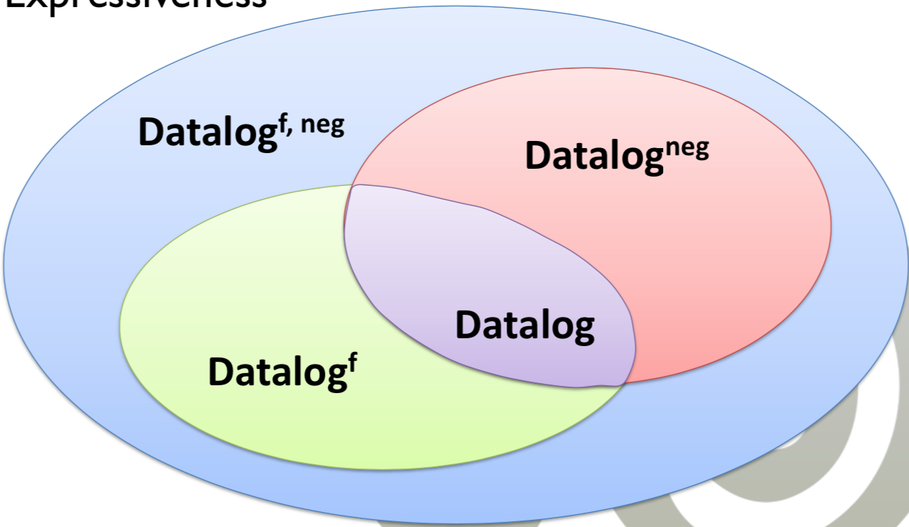
- Datalog program: Program with no functions and negative literals
- Datalog-neg program: With negative literals
- Datalog-f program: With functions
- Datalog-f,neg program: With functions and negative literals
- Classification by dependencies between predicates
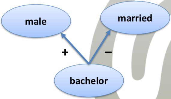
Program Connection Graph
- Idea:
- Find out the relation between predicates by examining their definitions
- Graph \( PCG(P) \) of program \( P \)
- Node: Predicate
- Directed edge \( (q, r) \): Definition of \( r \) contains \( q \)
- Positive edge: \( r \) occurs in positive literal
- Negative edge: \( r \) occurs in negative literal
- Recursive clique:
- Maximum subset of the predicates, between each pair of predicates exists a path
- Hierarchic program: No cycles in the PCG
- Recursive program: Cycles in the PCG
- Stratified program: Cycles in the PCG are only positive edges (negative edges are allowed, but not in the cycles)
Stratification
- Problem:
- If a predicate negatively depends on another predicate, the negative predicate does not limit the set of possible terms
- Idea:
- Layer a program \( P \) so that the definitions of negatively used predicates are already given
- Exclude the negation within recursion
Definition Stratification
- Stratification of program \( P \) is a disjoint partitioning \( P=P_1\uplus\ldots\uplus P_n \) into strata (parts)
- Order the predicates of a program \( P \): \( P=P_1...P_n \)
- If the definition of a predicate symbol \( P_i \) (head) depends on a positive body literal \( P_j \): \( i\leq j \)
- If the definition of a predicate symbol \( P_i \) (head) depends on a negative body literal \( P_j \): \( i > j \) (\( P_j \) must be before \( P_i \))
- e.g., \( even(x)\leftarrow \neg odd(x) \) (first define \( odd(x) \) before evaluating \( even() \))
- Program is stratified iff it has a stratification
Algorithm
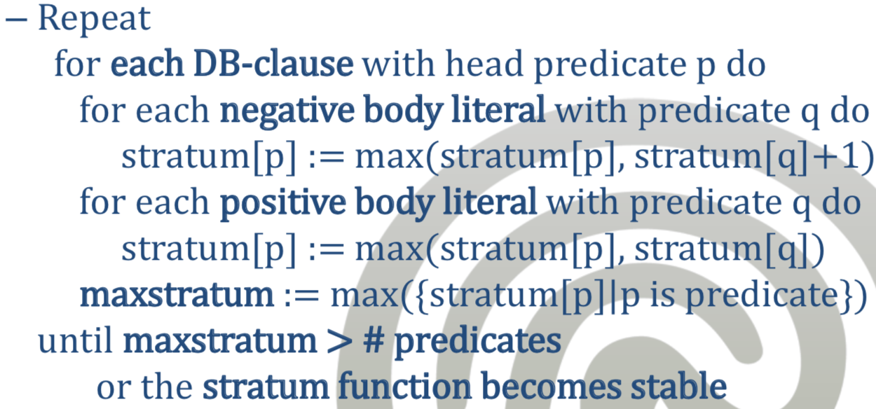
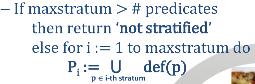
- Decidable
- Input: Set of DB-clauses/program \( P \)
- Output: Either a stratification or
not stratified - Idea:
- Iterate over all clauses and increase the stratum of a predicate if it depends on a negative literal
- Stop when the stratum does not change anymore or the maximal stratum exceeds the number of predicates (
not stratified)
Semantics
- Semantics
- What does a program a mean?
- How can a query be evaluated?
- Operative semantic:
- The semantic described by a state machine (production rule)
- Tilo: “Operative semantics means It does what we want it to do” (there is no natural semantics)
- Deductive systems:
- Prolog: Find truth values of the elements of the Herbrand universe
- e.g., SDL resolution
- Problem: Performance
- Datalog: Fixpoint iteration
- Sound and complete deductive system
- Idea: Iteratively compute all true ground facts
- Prolog: Find truth values of the elements of the Herbrand universe
- Datalog-f:
- Intended semantic: Least Herbrand Model
- Operative semantic: Fixpoint iteration
- Datalog-neg:
- Intended semantic: Perfect Herbrand Model
- Operative semantic: Iterated Fixpoint iteration
- Potentially unsafe (use Positive grounding)
- Potentially ambiguous (use Negation as failure (non-provided fact is assumed to be false))
- Problem:
- Naive operative semantics have suboptimal performance (Datalog-neg and Datalog-f)
Herbrand Models
- Goal:
- Check if a query and the DB-clauses are unsatisfiable
- Requires an operator for the semantic conclusion
- Requirements for the operator \( \vdash \):
- Find interpretation which is a model
- Decidable operator
- Efficient operator
- Sound: All generated atoms are true
- Complete: Generates all true atoms
- Use Herbrand interpretations (Datalog program consists of clauses)
- Idea:
- Facts are interpreted as true
- Fact rule
Q(x):-, i.e., \( \text{true}\rightarrow Q(x) \) - \( I(Q(x)) = \text{true} \) iff fact rule exists
- Always keep models containing these fact rules
- Fact rule
- Rules propagate truth values
- Propagate
trueiff premises aretrue B :- A1,...,An- \( I(B)=\text{true}\iff I(A_1,\ldots,A_n)=\text{true} \)
- Propagate
- Facts are interpreted as true
- Definition Semantic conclusion of a Datalog program
- \( \mathcal{P}\models W \)
- \( W \) is consequence of set of Datalog clauses if and only if each Herbrand interpretation satisfying each clause in \( \mathcal{P} \) also satisfies \( W \)
- Sound and complete
- Problem:
- Multiple models can satisfy the Datalog program
- Which model should be chosen?
Evaluation of Datalog-f
- Called Fixpoint Iteration
- Important:
- Find the least Herbrand Model \( M_\mathcal{P} \) of a Datalog program \( \mathcal{P} \)
- Problem:
- \( \mathcal{M} \) may be of infinite size
- Computing the intersection may be impossible
- Idea:
- Start with empty subset \( I_0 \) of Herbrand Base of logic language of the program
- This subset later identifies the Herbrand Interpretation
- Transformation \( T_\mathcal{P} \):
- Transformation rule \( T_\mathcal{P} \)
- \( I_{n+1}=T_\mathcal{P}(I_n) \)
- \( I_{n+1}=T_\mathcal{P}(...T_\mathcal{P}(T_\mathcal{P}(I_n))) \)
- Fixpoint iteration is a deductive system:
- Axioms: Program \( \mathcal{P} \)
- Deduction rule: Only \( T_\mathcal{P} \)
- Inferred ground fact \( W:\mathcal{P}\vdash W \)
- Purely syntactical deduction
- Closed World Assumption (everything that was not deduced is false)
Least Herbrand Model
- Definition Least Model:
- Herbrand model \( M \) is called least model iff \( M\subseteq M' \) for all other Herbrand Models \( M' \)
- Also called Intended Herbrand Model for Datalog-f
- This model is enforced by the program
- Evaluates facts/rules to true but nothing more
- Induces the Stable model semantics
- Always such a model exists (due to no negations)
- Lemma:
- Given:
- Datalog-f Program \( \mathcal{P} \)
- Set of all Herbrand models of \( \mathcal{P} \): \( \mathcal{M} \)
- Least Herbrand Model of \( \mathcal{P} \) \( \mathcal{M}_\mathcal{P}:=\bigcap \mathcal{M} \)
- \( M_{\mathcal{P}} \) is the intended semantics (other model possible)
- Given:
- Problem with Datalog-neg:
- Intersection can be empty
- e.g., \( \mathcal{P}=\{ Frog(x)\leftarrow \neg Toad(x)\} \): Models are \( \{Toad(Hector)\} \) or \( \{Frog(Hector)\} \)
Elementary Production
- Definition Elementary Production \( T_\mathcal{P} \)
- \( T_\mathcal{P}: 2^{B_\mathcal{L}}\rightarrow 2^{B_\mathcal{L}} \) (Map subsets of the Herbrand Base to subsets of the Herbrand Base)
- Idea: Forward chaining
- One-Step-Production (single iteration)
- Iteratively, add \( B \) from \( B\leftarrow A_1,\ldots,A_n \) iff \( \{A_1,\ldots,A_n\}\in T_\mathcal{P} \) and \( B \) is a ground instance
- Ground Instance: Quantifier-free sub-formula of a formula in prenex form where free variables are substituted with elements of the universe
- Evaluation of \( T_\mathcal{P} \) is monotonic
- \( I_n\subseteq I_{n+1} \)
- Set can only grow
- No negation can turn any formula false
- Fixpoint \( f \)
- \( \exists f\geq 0, \forall m\geq f:I_m=I_{m+1} \)
- Set is called stable (no changes after reaching the fixpoint)
- \( I_f \) is identified with the least Herbrand Model \( M_\mathcal{P} \)
- Minimal interpretation which is consistent with the program
Example
- Program \( \mathcal{P} \):
- \( edge(v_1,v_2). \)
- \( edge(v_1,v_3). \)
- \( edge(v_2,v_4). \)
- \( edge(v_3,v_4). \)
- \( path(x,y)\leftarrow edge(x,y). \)
- \( path(x,z)\leftarrow edge(x,y), path(y,z). \)
- \( I_0=\{\} \)
- \( I_1=\{edge(v_1,v_2),edge(v_1,v_3),edge(v_2,v_4),edge(v_3,v_4)\} \)
- \( I_2=I_1\cup\{path(v_1,v_2),path(v_1,v_3), path(v_2,v_4),path(v_3,v_4)\} \)
- \( I_3=I_2\cup\{path(v_1,v_4)\} \)
- \( I_4=I_3\cup\{\} \) (Fixpoint reached)
Operative Semantics
- Inferred ground fact \( W:\mathcal{P}\vdash W \)
- Result:
- Given a set of Datalog clauses \( \mathcal{P} \): \( \mathcal{P}\models W \iff \mathcal{P}\vdash W \)
- Corollary:
- If \( \mathcal{P} \) is finite, then the set of inferred ground facts from \( \mathcal{P} \) is finite
- Any Datalog model can be computed in finite space and time (a fixpoint must exist)
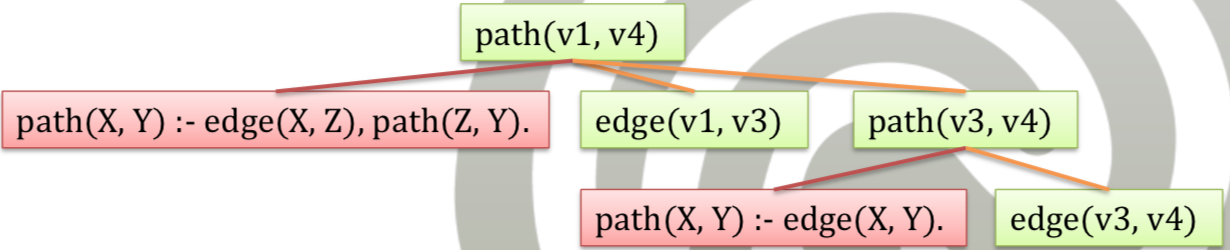
Definition Proof tree
- For each inferred ground fact \( W \), construct a proof tree
- Nodes:
- Fact nodes (inferred or existing)
- Rule nodes (rule from program)
- Root: \( W \)
- Proof tree shows minimal set of rules and facts required to infer \( W \)
- Tree height is minimal number of iterations to deduce \( W \)
- Lowest level corresponds to the first iteration
Soundness Theorem
- Each inferred ground fact \( \mathcal{P}\vdash W \) is a semantic conclusion \( \mathcal{P}\models W \)
- Proof:
- Induction over tree height
- Induction Base:
- Tree height is zero, then \( W\in\mathcal{P} \)
- \( W \) must be in each Herbrand model
- Thus, \( \mathcal{P}\models W \)
- Induction Step:
- Proof tree of depth \( i+1 \)
- There is a rule \( R\equiv B\leftarrow A_1,\ldots,A_n \)
- There are ground facts \( F_1,\ldots,F_n \)
- Rule and facts are at level \( i \)
- \( W \) can be inferred in one step by applying \( T_{\mathcal{P}} \) on \( R \) and \( F_1,\ldots,F_n \)
- \( F_1,\ldots,F_n \) are on level \( i \), so they have a proof tree with a depth at most \( i \)
- By induction hypothesis, \( 1\leq k\leq n:\mathcal{P}\models F_k \)
- Thus, each Herbrand model contains \( F_k\in I \)
- Since \( R\in I \), \( W\in I \) and \( \mathcal{P}\models W \)
Completeness Theorem
- Each semantic conclusion \( \mathcal{P}\models W \) is also an inferred ground fact \( \mathcal{P}\vdash W \)
- Proof:
- Assume the set \( \text{infer}(\mathcal{P}) = \{W|W\text{is ground fact}\land\mathcal{P}\vdash W\} \)
- Definition of \( \vdash \):
- Each fact \( F\in\mathcal{P} \) is deduced by \( \vdash \) (first iteration step)
- Thus, \( F\in\text{infer}(\mathcal{P}) \)
- Take rule \( R\equiv A\leftarrow B_1,\ldots,B_n\in\mathcal{P} \)
- Assume, there is a substitution \( \rho \)
- Such that the resulting ground facts can be concluded from the program
- \( \mathcal{P}\vdash \rho(B_1),\ldots,\rho(B_n) \)
- Then: \( \mathcal{P}\vdash\rho(A) \)
- \( \rho(A)\leftarrow\rho(B_1),\ldots,\rho(B_n) \)
- Thus, \( \rho(A)\in\text{infer}(\mathcal{P}) \)
- Then: \( \text{infer}(\mathcal{P}) \) is a Herbrand Model of \( \mathcal{P} \)
- Assume \( \mathcal{P}\models X \)
- Then: \( X \) must be in every Herbrand model of \( \mathcal{P} \)
- Conclusion:
- Since \( \text{infer}(\mathcal{P}) \) is a Herbrand model of \( \mathcal{P} \), it must hold that \( X\in\text{infer}(\mathcal{P}) \)
- Then: \( \mathcal{P}\vdash X \)
Query Execution
- Naive algorithm
- Given: Program \( \mathcal{P} \), Query \( Q \)
- Start the fixpoint iteration
- For each fact \( W \) with \( \mathcal{P}\vdash W \)
- If \( W\equiv \neg Q \) return the empty result set (check each fact)
- If \( W \) is ground instance of \( Q \), add \( W \) to the result set
- If fixpoint reached/set stable: Return result set
- Problem: Computation time (everything is re-computed)
Expressiveness
- Datalog-f has operative semantics
- Theorem: Datalog-f is Turing-complete
- Thus, negation is not required
- But: Negation is very intuitive and user-friendly
Evaluation of Datalog-neg
- Nice feature: Express negation (e.g., specify a workday)
- Problems with negation:
- Least Herbrand Model might not exists (intersection of Herbrand models)
- Soundness and completeness of fixpoint iteration does not hold anymore
- Datalog-neg program has multiple minimal models
Constraints
- Use stratification!
- Problems:
- Unsafe rules
- Ambiguous models
- Definition Unsafe rule:
- e.g., \( P(y)\equiv \neg R(y) \)
- Negation builds the complement set
- The complement of a finite set in an infinite universe is infinite
- Thus, all universe ground terms must be tested
- Problem: Usually, \( R(y) \) is true for a small subset of the Herbrand Universe, to there are a lot of \( P(y) \) in the model (storage overhead)
- Ambiguous model:
- e.g., \( P(y)\equiv \neg R(y) \)
- If no information about \( R(y) \) is in the Datalog program, is \( P(y) \) true or not?
- Open World Assumption
- Use constraints:
- Safe negation: If variable appears in a negative literal, is must appear in positive literal in the body
- Restrict to finite universe
- Variable must be grounded
- Positive grounding:
- First evaluate the positive literals, then the negative literals
- Restrict to finite set
- Use a limited number of candidate terms
- Evaluation is performed stratum-wise
- Positive facts in lower strata restrict the set of possible terms
- Safe negation: If variable appears in a negative literal, is must appear in positive literal in the body
Minimal Model
- Model for Datalog-neg programs
- Definition Minimal model
- A Herbrand model \( M \) is minimal iff there is no other Herbrand Model \( M' \) such that \( M'\subset M \)
- Induced semantics: Minimal Herbrand Semantics
- Open problem:
- What is the intended semantics?
- Which model should we choose?
- Requirement:
- Deterministic decision criteria to use an appropriate/intended model
- Idea: Use stratification
- Order predicates into a hierarchy
- Execute only stratified programs (it is not possible to execute non-stratified programs)
Perfect Model
- Model for Datalog-neg programs
- Idea:
- Create a preference between the minimal models
- Based on the degree of stratification
- Priority Relation \( <_\mathcal{P} \)
- Relation on elements of Herbrand Base
- Based on negative dependencies and the level of stratification
- \( P(t_1,\ldots,t_n)<_\mathcal{P}Q(s_1,\ldots,s_m) \) iff there is a negative edge from \( P \) to \( Q \) in the PCG of \( \mathcal{P} \)
- e.g., \( P \) has lower priority than \( Q \), use \( Q \) first
- Lemma: If Program \( \mathcal{P} \) is stratified,\( <_\mathcal{P} \) is an irreflexible partial order
- Preference relation \( \leq \)
- Between two minimal models \( \mathcal{M}_1 \) and \( \mathcal{M}_2 \)
- Based on the priority relation
- \( M_1\leq M_2 \) iff
- \( \mathcal{M}_1 = \mathcal{M}_2 \)
- OR \( \forall A\in\mathcal{M}_1\setminus\mathcal{M}_2: \exists B\in\mathcal{M}_2\setminus\mathcal{M}_1: A <_\mathcal{P} B \)
- e.g., prefer \( \mathcal{M}_1 \) if all elements of \( \mathcal{M}_1 \) which are not in \( \mathcal{M}_2 \) are preferred
- Definition Perfect model:
- \( \mathcal{M} \) is perfect model iff \( \mathcal{M}\leq \mathcal{M}' \) for all \( \mathcal{M}' \) of \( \mathcal{P} \)
- Theorem:
- For each Datalog-neg program, there exists a perfect model which is also a minimal model
- Intended semantics of a Datalog-neg program is defined by this perfect and minimal model
- Result:
- Requirement to modify the fixpoint iteration
- Negation as Failure semantics: First evaluate positive literal, then the negative
Iterated Fixpoint Iteration
- Elementary Production \( T_\mathcal{P}^J \)
- \( T_\mathcal{P}^J:2^{B_\mathcal{L}}\rightarrow 2^{B_\mathcal{L}} \)
- Production rule depends on the set \( J \)
- Incrementally add ground instance \( B \) with \( B\leftarrow A_1,\ldots,A_n,\neg C_1,\ldots,\neg C_m \) with \( \{A_1,\ldots,A_n\}\subseteq I \) and \( \forall 1\leq i \leq m: C_i\notin J \)
- Iterated Fixpoint Iteration
- Using stratification
- Use Elementary Production inside each stratum until the fixpoint is reached, then go to the next stratum
- Evaluate strata-wise
- Program \( \mathcal{P}=\mathcal{P}_0\cup\ldots\cup\mathcal{P}_n \)
- \( I_0=T_{\mathcal{P}_0}(\emptyset) \)
- \( I_1=T_{\mathcal{P}_0\cup\mathcal{P}1}(T^{I_0}_{\mathcal{P}_1\cup I_0}) \)
- Informally
- Apply elementary production rule to each stratum
- After the first stratum, the set contains all facts that can be derived from that stratum
- For the higher strata, to check \( \neg P(a) \) only check if \( P(a) \) is already in the set
- Theorem:
- The Iterated fixpoint \( I_n \) is the minimal perfect Herbrand model of \( \mathcal{P} \)
- Result: Iterated Fixpoint iteration is a computable operative semantic for Datalog-neg
Implementation
- Question:
- How to implement the elementary production operator?
- How to store the extensional database?
- Idea:
- Use relational databases (do not implement from scratch)
- Use database features
- Map Datalog-neg to Relational Algebra
- e.g., merge Datalog-reasoning with relational database
- Implements the Bottom-up approach
Relational Algebra
- Facts are stored in relations
- Relation
- \( R\subseteq D_1\times\ldots\times D_n \)
- Domains \( D_i \) are finite
- Operators:
- Base: \( \times, \sigma, \pi, \cup, \setminus \)
- Derived: \( \Join, \ltimes, \rtimes \)
- Different notation:
- Attributes are referenced by number, e.g.
#1 - Relations can be referenced by
left, right
- Attributes are referenced by number, e.g.
- Types of RA:
- \( \text{RelAlg}^+ \): Excluding the set minus operator
- \( \text{RelAlg} \): Including the set minus operator (more expressiveness)
Fixpoint Iteration
- Only consider safe Datalog-neg programs (positive grounding)
- Task:
- Store extensional DB in relations
- Encode intensional DB in relational algebra and the elementary production operator
- Facts:
- Extensional database predicates \( r_1,\ldots,r_m \) are assigned to relations \( R_1,\ldots,R_m \)
- Rules:
- Intensional database predicates \( q_1,\ldots,q_m \) are assigned to relations \( Q_1,\ldots,Q_m \)
- Relations \( Q_1,\ldots,Q_m \) are filled during evaluation
- Predicate definition:
- Predicate is either defined on extensional or intensional database
- Does not limit expressiveness, but increases readability
- Operators \( <,>,\leq,\geq,=,\neq \)
- Are assigned to hypothetical relations
LT, GT, ... - Are not stored (infinite size)
- Later, can be removed
- Are assigned to hypothetical relations
- Mapping:
- Relational Algebra to Datalog
- Datalog to Relational Algebra
- Datalog-f uses \( RelAlg^+ \)
- Datalog-neg uses \( RelAlg \) (due to the set minus operator)
- Elementary production operator corresponds to \( eval(C) \)
Mapping Relational Algebra to Datalog
- \( \sigma_{\#=5}\equiv R(X, 5). \)
- \( \pi_{\#1}R\equiv R'(X)\text{ :- }R(X,Y). \)
- \( R\times S\equiv RS(W,X,Y,Z)\text{ :- }R(W,X), S(Y,Z). \)
- \( R\bowtie_{[left].\#1=[right].\#2}S\equiv RS(W,X,Y,Z)\text{ :- }R(W,X),S(Y,Z),W=Z. \)
- \( R\cup S \)
- \( \equiv R'(X,Y)\text{ :- }R(X,Y). \)
- \( \equiv R'(X,Y)\text{ :- }S(X,Y). \)
- \( R\setminus S\equiv R'(X,Y)\text{ :- }R(X,Y), \neg S(X,Y). \)
Mapping Datalog to Relational Algebra
- Goal:
- Transform Datalog rule to Relational Algebra
- Transform \( C\equiv R\text{ :- }L_1,\ldots, L_n \)
- Steps:
- Pre-processing of predicates
- Transformation of each literal
- Composition of literal transformations to an expression
Pre-Processing
- Rules are transformed, so that the head contains only variables
- Replace constant with variable
- Add literal binding the variable to the constant
- e.g.,
q(X, a) :- L1(X, a) - e.g.,
q(X, Y) :- L1(X, Y), Y=1
- Order literals to ensure safety
- Literal is unsafe it is potentially infinite
- Positive body literals must be before negative literals (positive grounding, stratification)
- e.g.,
R(X,Y) :- X=Y, p(X), q(Y)(X=Yis unsafe) - e.g.,
R(X,Y) :- p(X), q(Y), X=Y(Xis grounded)
Literal Transformation
- Task:
- Transform literal \( L_i \) to relational expression \( E_i \)
- Atomic component of literal:
- \( A_i\equiv p_i(t_1,\ldots,t_m) \)
- \( p_i \) is respective predicate
- Transform \( A_i \) to \( E_i\equiv \sigma_\theta (P_i) \)
- Relation \( P_i \) corresponds to \( p_i \)
- Selection criterion \( \theta \) is conjunction of conditions for each term \( t_i \)
- \( \#i = t_i \) if \( t_i \) is constant
- \( \#i = \#j \) if terms \( t_i \) and \( t_j \) are the same variables
- e.g., \( R(X,X,Y,2)\rightarrow \sigma_{\#1=\#2\land \#4='2'} \)
Composition
- Task:
- Compose relational expression \( E_1, \ldots, E_k \) to body expression \( F \)
- Steps (From left to right):
- Initialization: \( F_1 := E_1 \)
- Cases (\( F_2,\ldots,F_k \)):
- \( L_i \) does not contain any variables of the previous body literals
- i.e., \( vars(L_1,\ldots,L_{i-1})\cap vars(L_i)=\emptyset \)
- \( F_i := F_{i-1}\times E_i \)
- Resulting in Cartesian product
- e.g.,
R(X,Y):- q(X), r(Y)–> \( F_2=Q\times R \) - Conjunction of unrelated body literals results in cartesian product
- \( L_i \) is positive and shares variables with the previous body literals
- \( F_i := F_{i-1}\Join_\theta E_i \)
- Condition \( \theta \) enforces equality of shared variables
- e.g., \( \bowtie_{[left].\#2=[right].\#1} \)
- Conjunctions of related positive literals result in a join
- \( L_i \) is negative and shares variables with the previous body literals
- \( F_i:=F_{i-1}\setminus (F_{i-1}\ltimes_\theta E_i) \)
- Condition \( \theta \) enforces equality of shared variables
- e.g., \( R(X)\text{ :- }q(x),\neg r(X) \)
- \( E_1:=F_1=Q \)
- \( E_2=R \)
- \( F_2=Q\setminus (Q\ltimes_{Q.\#1=R.\#1}R) \)
- Conjunctions of related negative literals result in a set-minus
- \( L_i \) does not contain any variables of the previous body literals
- Hypothetical relations
- \( LT, GT, LTE, GTE, EQ, NEQ \)
- Replace with the arithmetic operators in a \( \sigma_\theta \)
- Result:
- Datalog rule: \( C\equiv R\text{ :- }L_1,\ldots, L_n \)
- \( eval(C) = \pi_{vars(R)}(F) \)
- \( eval(q_i)=\bigcup_{C\in def(q_i)}eval(C) \) (multiple rules for a predicate)
- e.g.,
path :- edgeandpath :- edge, path
- e.g.,
- Elementary production rule \( T_{\mathcal{P}} \) corresponds to evaluating \( eval(C) \)
Example
- \( R(X,Y)\text{ :- }X<Y,q(3,X),r(Y) \)
- Preprocessing:
- \( R(X,Y)\text{ :- }q(3,X),r(Y),X<Y \)
- Literal transformation:
- \( E_1=\sigma_{\#1=3} Q \)
- \( E_2=R \)
- \( E_3=LT \)
- Composition:
- \( F_1=E_1=\sigma_{\#1=3} Q \)
- \( F_2=F_1\times E_2=\sigma_{\#1=3} Q\times R \)
- \( F_3=(\sigma_{\#1=3} Q\times R)\bowtie_{[left].\#2=[right].\#1\land [left].\#3=[right].\#2} LT \)
- Arithmetic operators:
- \( F_3=\sigma_{\#2<\#3=[right].\#2}(\sigma_{\#1=3} Q\times R) \)
- Optimization:
- \( F_3=(\sigma_{\#1=3} Q)\bowtie_{\#2<\#3=[right].\#2} R \)
Algorithm
- Preparation:
- Create relations for extensional predicates \( p_i \) and store facts in it
- Create relations for each intensional predicate \( q_i \) (empty)
- Execute elementary production (run \( eval(q_i) \)) and store results temporally (temp-table)
- If IDB relations have not changed, fixpoint is reached
- Else: Replace intensional predicate relations with the current temp-table
- GOTO (2)
- Run the query on all relations
Evaluation Strategies
- Evaluation strategies:
- Bottom-Up
- Top-Down
- Bottom-Up
- Strategy:
- Start with the EDB facts
- Generate new facts
- Then, discard all facts not matching the query
- Forward-chaining (done by fixpoint iteration)
- Pro:
- Good in restricted and small scenarios
- Con:
- Massive overhead (generating all facts, only selecting a small subset)
- e.g. all facts in EDB, query contains only rules (optimized by Magic Sets)
- Strategy:
- Top-Down
- Strategy:
- Start with the query
- Generate proofs to the EDB facts
- Usually, done by logical programming environments
- e.g., SDL resolution
- Backward-chaining
- Pro:
- Good in complex scenarios (where Bottom-Up is restricted)
- Strategy:
Top-Down Approach
- Idea:
- Query \( Q\equivpp(t_1,\ldots,t_n) \)
- Iteratively general all proof tree starting with a known fact and ending with a ground instance of \( Q \)
- Iteration is performed over the tree depth
- Helper data structure: Search trees
- Search trees are transformed to proof trees
- Stop if all proof trees are generated
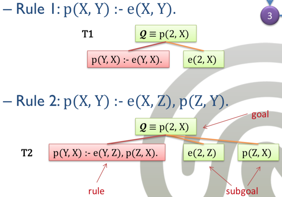
- Definition Search Tree:
- Generic Proof Tree which is parameterized (with placeholders)
- Leafs called subgoal nodes
- Root called goal node
- Generate proof trees from search trees
- Definition Full proof tree:
- Proof tree having only ground facts in all leaf nodes
- Unifiable of query and rule:
- Head predicate of the rule is the same as the query
- Generation strategies (search and proof trees):
- Level-saturation strategy
- Breadth-first approach
- Generate search tree one by one depth
- Rule-saturation strategy
- Depth-first approach
- Level-saturation strategy
Naive Algorithm
- Approach: Level-saturation strategy
- Query \( Q\equiv p(t_1,\ldots,t_n) \)
- Note:
- Backward-chaining can generate all proof trees
- This type of backward-chaining only generates proof trees with grounded facts in the leaf nodes
- Theorem:
- For each proof tree matching the query, there is a respective full proof tree
- Performance:
- Far from optimal
- Algorithm generates all possible search and proof trees with worst-case depth
Search Tree Generation
- Construct a search tree with \( Q \) as root
- Take a rule:
- \( R\equiv H\leftarrow A_1,\ldots,A_k \) from \( \mathcal{P} \)
- Attach \( R \) as rule node
- Attach the \( k \) subgoal nodes (body predicates \( A_1,\ldots,A_k \))
- Unify them (replace by the given variables of the root)
- IF all leaf nodes are goal nodes: GOTO (1) and choose a different role
- ELSE: Repeat procedure with each subgoal rule nodes 4. Attach a new level 5. Treat the subgoal nodes as new root
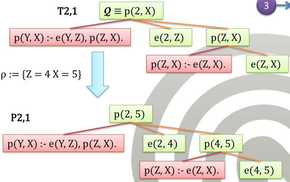
Proof Tree Generation
- Take a search tree
- Find substitution \( \rho \):
- For each goal node \( C \)
- \( \rho(C)\in P\cup EDB \)
- Substitution turns the search tree into a valid proof tree
- Then, the root node is a result of the query
Example

Stopping Criterion
- Problem:
- Using recursive rules, the proof tree can have an infinite depth
- At which height do we stop?
- Limitation:
- Datalog program and EDB are finite
- Useful combinations of facts and predicates are finite
- For each predicate symbol at each position there can be substituted any constant symbol (making it finite)
- Theorem:
- Backwards-chaining remains complete if the search depth is limited to \( \text{#pred} \cdot \text{#const}^{\max(args)} \)
- \( \max(args) \): maximal arity of all predicates
- Provides an upper bound for backward chaining
- Proof:
- Only consider syntactically interpreted facts
- Limited number of ground facts -> limited number of levels
Resolution
- Robinson, 1965
- Technique for refutation theorem proofing (reductio ad absurdum)
- The standard technique for logical symbolic computation
- Multiple variants
- Most popular: SDL resolution
- Selective Linear Definite clause resolution
- e.g., by languages like Prolog and Lisp
Recursive SQL (D)
- Most applications use SQL
- SQL2 (SQL-92) no really usable recursive queries
- SQL3 (SQL-99) adds new features to SQL
- BLOBs
- Soft constraints
- Updatable views
- Active databases
- UDF, UFT, UDM
- References
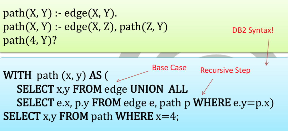
- Recursive Temporary Tables
- DB2: Common Table Expressions (CTE)
- Idea:
- Predicate represented in temporary table
- Definition consists of two parts:
- Base case (EDB of predicates)
- Recursive step (IDB)
- Keyword:
WITH - Linear recursion:
- Recursive steps may one use its own table once
- Counterpart: non-linear recursion
- CTE support negation
- Similar restrictions as in Datalog
- Statements must be stratified
Optimization
- Motivation:
- Fixpoint-algorithms have a bad performance
- Idea:
- Skip unnecessary steps and terminate earlier (save time)
- Logical Rewriting:
- Magic Sets
- Counting
- Static Filtering
- Algebraic Rewriting:
- Push Selection
- Variable reduction
- Constant reduction
- Bottom-Up evaluation:
- Naive (Jacobi, Gauss-Seidel)
- Semi-naive (Delta Iteration)
- Henschen-Naqvi
- Top-Down evaluation:
- Naive
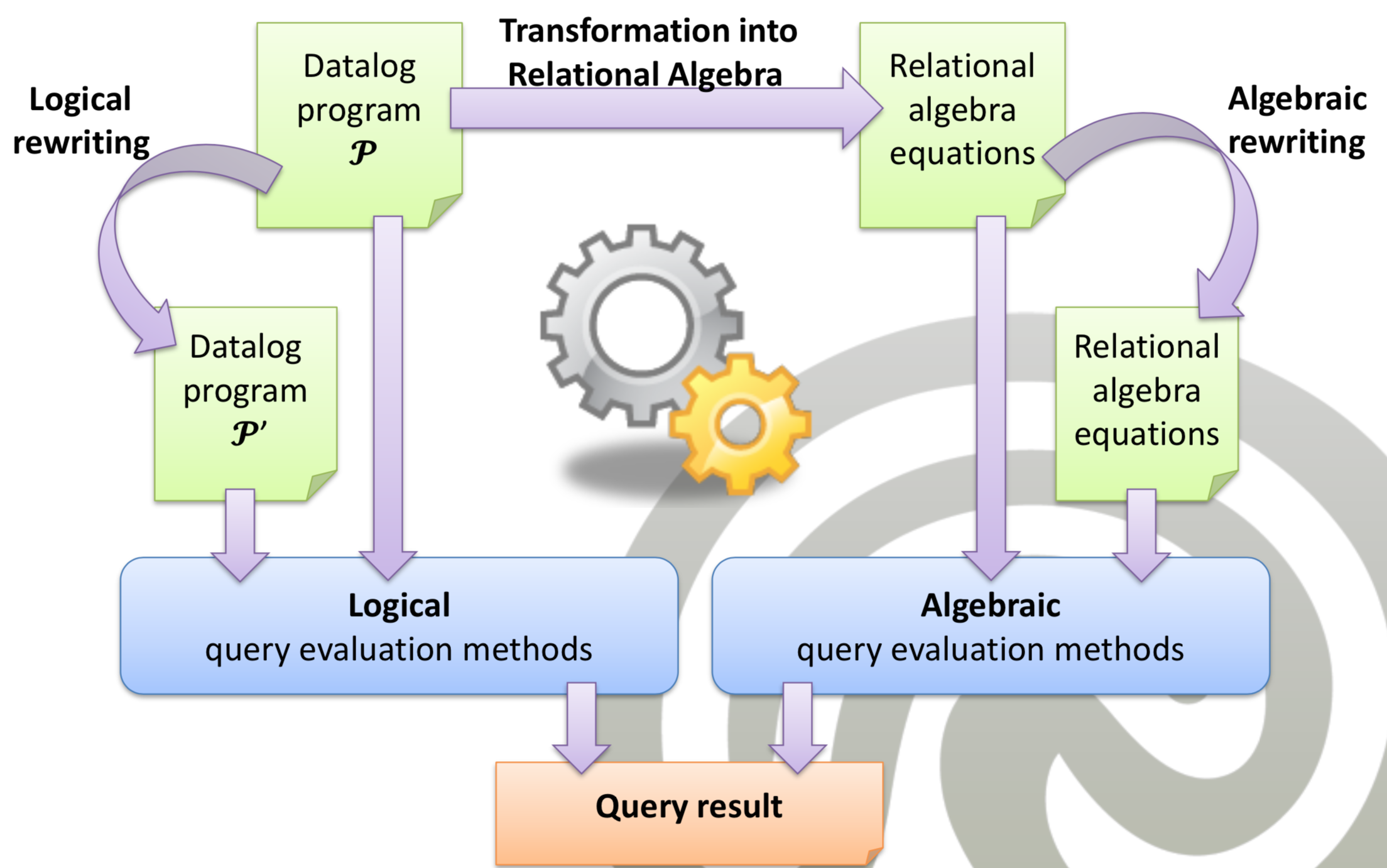
Classification of Evaluation Algorithms
- Search technique
- Bottom-up vs. top-down
- Formalism
- Logical vs. algebraic
- Objective
- Rewriting vs. optimization
- Traversal Order
- Breath-first vs. depth-first
- Approach
- Syntactic vs. semantic
- Structure
- Goal vs. rule
Search Technique
- Bottom-Up
- Forward-chaining of rules (using the EDB)
- Result set is subset of all generated facts
- Set-oriented approach (good for DBs)
- Top-Down
- Backward-chaining of rules
- Start with query, construct proof tree
- Result set is generated tuple-by-tuple
- Less suitable for DBs (not set-oriented)
Formalism
- Logical and algebraic are non-exclusive
- Logical
- Datalog program as logical rules
- Connection of query predicate and rule predicates
- Algebraic
- IDB corresponds to a system of algebraic equations
- cf. Relational Algebra Optimization
Objectives
- Program rewriting and evaluation optimization are non-exclusive
- Program Rewriting
- Rewrite program \( \mathcal{P} \) to semantically equivalent program \( \mathcal{P}' \)
- \( \mathcal{P}' \) can be executed faster using the same evaluation method
- e.g., Magic Sets algorithm
- Evaluation Optimization
- Improve process of evaluation itself
- e.g., Gauss-Seidel Iteration, Delta Iteration
Traversal Order
- Affects evaluation order of predicates in the body
- Depth-First
- Evaluate body in order with depth-first
- Performance may depend on the order
- Breadth-First
- Evaluate the body predicates at the same time
- Search tree grows balanced
Approach
- Syntactic:
- Focus on syntax of rules
- Easier, more popular than semantics
- Semantic:
- Use external knowledge for evaluation
- e.g., integrity constraints
- Use external constraints to improve performance
Structure
- Rule Structure
- Goal Structure
Bottom-Up Evaluation
- Bottom-up evaluation is easy
- Bottom-up evaluation techniques are usually based on the fixpoint iteration
- Start with empty initial solution \( X_0 \)
- Use production rule \( T \): \( X_{n+1}=T(X_n) \)
- If \( X_{n+1}=X_n \), fixpoint is reached
- Operative implementation types:
- Full enumeration (generate all instances are then reject the wrong ones)
- Restricted enumeration (generate instances based on a given set of ground instances)
Jacobi-Iterations
- Class of most naive fixpoint algorithm
- Solve \( Ax=b \) linear equation systems
- Characteristics:
- Intermediate result \( X_{n+1} \) is computed solely by using all data of \( X_n \)
- No use of intermediate results
- Complexity of iteration step: \( |X_n|\cdot|X_{n+1}| \)
- Elementary production rules and the naive fixpoint iteration are Jacobi Iterations
- Disadvantage:
- In each iteration, all facts of the previous iteration are deduced again
Gauss-Seidel Iterations
- Idea:
- Respect intermediate results of Jacobi Iteration
- Use Information created in current iteration directly
- Modify the elementary production rule
- Gauss-Seidel Production Rule:
- Additional: \( ...\{A_1,\ldots,A_n\}\subseteq I\cup \text{newBs} \)
- Use newly generated head instances from \( \text{newBs} \) directly
- Improves convergence speed
- Effectiveness depends on the order of evaluation
- e.g., first
edge, thenpath
- e.g., first
- Problem: Still recomputes all known facts
Semi-Naive Iteration
- Motivation:
- Jacobi and Gauss-Seidel Iterations compute a lot of facts
- Idea:
- Elementary production is strictly monotonic
- \( I_i\subseteq I_{i+1} \)
- Therefore: Only compute new facts per iteration
- New facts involve new facts from the last iteration step
- Elementary production is strictly monotonic
Delta-Iteration
- Difference between two steps: \( \Delta I_i \)
- Reminder: \( I_{n+1}=T_{\mathcal{P}}(I_n) \)
- \( \Delta I_i=I_i\setminus I_{n-1} \)
- \( \Delta I_1:=I_1\setminus I_0=T_{\mathcal{P}}(\emptyset) \)
- \( \Delta I_{n+1}:=I_{n+1}\setminus I_n \)
- \( = T_{\mathcal{P}}(I_n)\setminus I_n \)
- \( = T_{\mathcal{P}}(I_{n-1}\uplus \Delta I_n)\setminus I_n \)
Auxiliary Function
- Important:
- Efficiently compute \( \Delta I_{i+1}=T_{\mathcal{P}}(I_{n-1}\uplus \Delta I_i)\setminus I_i \)
- Problem:
- Usually, \( T_{\mathcal{P}} \) is inefficient, because applied in all rules in the EDB
- Idea: Use auxiliary function
- \( aux_{\mathcal{P}}:2^{B_{\mathcal{P}}}\times 2^{B_{\mathcal{P}}}\rightarrow 2^{B_{\mathcal{P}}} \)
- Auxiliary function should generate the new knowledge
- i.e., the recursive parts of the rules
- only they generate new knowledge
- i.e., \( T_{\mathcal{P}}(I_{n-1}\uplus \Delta I_i)\setminus I_i = aux_{\mathcal{P}}(I_{n-1}, \Delta I_i)\setminus I_i \)
- Classic method: Symbolic differentiation
- e.g., derivation rules from school
Symbolic Differentiation
- Symbolic differentiation operator \( dF \)
- Apply on relational algebra expressions (transform Datalog program)
- Relations:
- \( dF(E) = \Delta R \) if \( E \) is an IDB relation \( R \)
- \( dF(E) = \emptyset \) if \( E \) is an EDB relation \( R \) (no change)
- Selection/Projection:
- \( dF(\sigma_\theta(E))=\sigma_\theta(dF(E)) \)
- \( dF(\pi_L(E))=\pi_L(dF(E)) \)
- Set operations:
- \( dF(E_1\cup E_2)=dF(E_1)\cup dF(E_2) \)
- Cross product/Join:
- \( dF(E_1\times E_2)=E_1\times dF(E_2)\cup dF(E_1)\times E_2\cup dF(E_1)\times dF(E_2) \)
- \( dF(E_1\bowtie_\theta E_2)=E_1\bowtie_\theta dF(E_2)\cup dF(E_1)\bowtie_\theta E_2\cup dF(E_1)\bowtie_\theta dF(E_2) \)
Example
- Program:
anc(X,Y) :- par(X,Y).anc(X,Z) :- par(X,Y), anc(Y,Z).
- Relational algebra expression:
- \( anc\equiv par\cup \pi_{\#1,\#2}(par\bowtie_{\#2=\#1} anc) \)
- Symbolic differentiation:
- \( dF(par\cup \pi(par\bowtie anc)) \)
- \( =dF(par)\cup dF(\pi(par\bowtie anc)) \)
- \( =\emptyset\cup \pi(dF(par\bowtie anc)) \)
- \( =\pi(dF(par)\bowtie anc\cup par\bowtie dF(anc)\cup dF(par)\bowtie dF(anc)) \)
- \( =\pi(\emptyset\cup par\bowtie dF(anc)\cup \emptyset) \)
- \( =\pi(par\bowtie \Delta anc) \)
- Result: Operator computing only the new results
Algorithm
- Initialization:
- \( I_0:=\emptyset \)
- \( \Delta I_1=:T_P(\emptyset) \)
- \( i:=1 \)
- Iteration until \( \Delta I_{i+1}=\emptyset \):
- \( I_i:=I_{i-1}\uplus \Delta I_i \)
- \( \Delta I_{i+1}:=aux_P(I_{i-1}, \Delta I_i)\setminus I_i \)
- \( i:=i+1 \)
- Fixpoint: \( I_k \) (where \( I_k=I_{k-1} \))
- Note: For stratified programs, execute per stratum
- The \( \setminus \) is required because it can happen that we re-compute some facts if we have a circle (otherwise we would miss the fixpoint)
Algebraic Rewriting (Push Selection)
- Here: Push Selection
- Transform Datalog program to relation algebra
- Use RA optimizations (like in RDB2)
- Use Push Selection
- Push selection down in the Query Tree
- Prevent large intermediate results
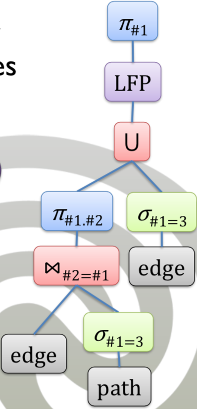
- Least fixpoint iteration:
- LFP operator
- Apply \( LFP \) on query predicate
- \( ?anc(X, 3) \)
- \( \pi_{\#1} \sigma_{\#2=3} LFP(par\cup anc) \)
- Problem:
- Push Selection is not trivial
- Can not be easily interchanged with the LFP operator
- Example:
- Rule:
path(x,y) :- edge(x,z), path(z,y) - Query:
?path(3,y)(bindx=3) - Resulting expression: \( \pi_{\#2} \sigma_{\#1=3} LFP(path) \)
- Pushing down the selection \( \sigma_{\#1=3} \) before \( path \) would affect the \( path \) from the rule
- Thus, the variable \( z \) would be falsely be bound
z=3
- Rule:
- When to re-order LFP operator and selection?
- Predicate \( P(X_1,\ldots,X_i,\ldots,X_n) \)
- Query \( ?P(t_1,\ldots,c,\ldots,t_n) \)
- Query binds the variable \( X_i \) (i-th position) to constant \( c \) (\( X_i=c \))
- Criterion:
- Selection \( \sigma_{\#i=c} \) and \( LFP \) can safely be interchanged if \( X_i \) occurs in all literals with predicate \( P \) on the i-th position
Logical Rewriting
- Logical rewriting:
- Transform program \( \mathcal{P} \) to a semantically program \( \mathcal{P}' \) which can be evaluated fast with the same technique
- Same result, but faster evaluation using Jacobi Iteration
- Here: Magic Set Algorithm
Magic Sets
- Idea:
- Un-intuitive but effective rewriting strategy
- Rewriting method to exploit syntactic form of the query
- Transfer binding patterns from top-down search trees into rewriting
- e.g., query
?ancestor(Tilo, X) - Perform potentially useful deductions
- Problem:
- Propagating bindings (e.g., X=Tilo) does not work always
- Binding more difficult for rewriting than for two-down evaluation
- Magic Set Strategy:
- Rules are augmented with additional constraints (modeled via the magic predicate)
- Bind variables to members of the magic set
- Predicates are adorned to restrict the search space (en. “schmücken/verzieren”)
- Use Sideways information passing:
- Send information of sub-expressions not only to parent but also to other correlated part
- Used to propagate the binding information
- Used in several database systems
- i.e., clever re-ordering of the body literals
- Overview:
- Query is part of the program
- Use reachable adorned system (all necessary predicates)
- Create magic set for each original predicate (using magic rules and magic predicates)
- Result: Restrict original rules
Definitions
- Query (goal)
- Rewrite the query as rule and add to program
- e.g.,
?ancestor(Tilo, X)asq(X) :- ancestor(Tilo, X)
- Distinguished arguments
- Distinguish arguments of predicates (distinguished or not distinguished)
- Distinguished: Range is restricted by either constants within the same predicate or variables which already restricted
- An argument is distinguished iff
- if is a constant
- OR it is bound by an adornment
- OR it is in some EDB fact with any distinguished argument
- Distinguished predicate
- A Predicate occurrence is distinguished if all of its arguments are distinguished
- e.g., EDB facts are always distinguished
- Predicate is adorned/annotated to express which arguments are distinguished
- As many adornments as variables in the predicate
- In some rules, variables are bound, in other they are free
- Types of adornments (per argument):
- \( b \): bound (distinguished variable)
- \( f \): free (non-distinguished variable)
- e.g., \( P^{fb}(X,2) \)
- Important: Each adorned predicate is treated as an own predicate with its own rules
- There are \( 2^n \) possible adornments for an n-ary predicate
Workflow
- Rewrite query to a rule
- e.g., \( ?anc(X, Tilo). \)
- \( \rightarrow q(X) \text{ :- } anc(X, Tilo). \)
- e.g., \( ?anc(X, Tilo). \)
- Create the reachable adorned system
- Start with the query
- Adorn predicates occurring in the query
- EDB facts are not adorned
- Create Magic Program:
- Create magic predicates:
- Generate magic predicates for each adorned predicate
- Create magic rules:
- Drop free variables, keep constants
- Create rules \( magic\_p\_\beta\leftarrow magic[A]\land\ldots \)
- Remove old rules
- Create magic predicates:
- Return the Magic program
Reachable Adorned System
- Program that contains all reachable facts (answers to the query)
- i.e., find the required adorned predicates
- Remember: there are \( 2^n \) possible adorned predicates
- Replace original predicates with respective adornments
- Only adorn IDB rules
- Steps:
- Start with query (\( r=0 \))
- e.g., \( q^f(X) \text{ :- } anc^{fb}(X, Tilo). \)
- Recursively, continue with the new adorned predicates
- e.g., \( anc^{fb}(X,Y)\text{ :- }par^{ff}(X,Z),par^{fb}(Z,Y). \)
- e.g., \( par^{fb}(X,Y)\text{ :- }mother(X,Y). \)
- Start with query (\( r=0 \))
- Adornment rule ():
- Predicate \( A\equiv p(t_1,\ldots,t_n) \)
- Adornment pattern \( \beta \) (e.g.,
bf) - \( adorn(A,\beta):=p\_\beta(t_1,\ldots,t_n) \) (if \( p \) is IDB rule and not \( query \))
Magic Rule
- Each adorned predicate has its own defining rule (here, the attributes are restricted)
- Goal: Magic rules add interesting constants to the magic set
- Definition Magic Predicate:
- Magic Predicate defines a magic rule
- Literal \( A\equiv p\_\beta(t_1,\ldots,t_n) \) with adornment \( \beta \)
- \( magic[A]:=magic\_p\_\beta(t_{i_1},\ldots,t_{i_k}) \)
- \( 1\leq i_1\leq ...\leq i_k\leq n \) where \( t_{i_j} \) is bound in \( \beta \)
- i.e., drop the free terms, keep the bound terms
- Exception is the query predicate \( q \):
- \( magic[q]=true \)
- e.g. \( P^{fb}(X,Tilo) \equiv \text{magic_P_b}(Tilo) \)
- Generate modified rules:
- Idea: Restrict original rule by adding the magic predicates to the rule
- Create for each IDB rule
- Take adorned IDB rule \( A\leftarrow B_1,\ldots,B_n \)
- Modified rule: \( A\leftarrow magic[A]\land B_1,\ldots,B_n \)
- Generate magic rules:
- Idea: Restrict search space of the original rule
- Create a magic rule (for each adorned rule of an IDB predicate):
- Take adorned rule \( A\leftarrow B_1,\ldots,B_n \)
- For each \( 1\leq i\leq n \) with \( B_i \) is IDB rule
- Magic rule: \( magic[B_i]\leftarrow magic[A]\land B_1\land ...\land B_{i-1} \)
- Rule name is derived from the original rule
- e.g., \( q^f(X)\text{ :- }anc^{fb}(X, Tilo). \)
- Result: \( \text{magic\_r0\_anc}(Tilo)\leftarrow true. \)
- e.g., \( anc^{bf}(X,Y)\text{ :- }par^{bf}(X,Z),par^{ff}(Z,Y). \)
- Result: \( magic\_par\_bf(X)\leftarrow magic\_anc\_bf(X). \)
- ~~This creates multiple magic predicates for a single adorned predicate~~
- ~~Because the name is derived from the rule number~~
- ~~Create a predicate for combining all predicates from the different rules~~
- ~~e.g.~~
- ~~\( magic\_anc^f(X)=magic\_r0\_anc(X). \)~~
- ~~\( magic\_anc^f(X)=magic\_r2\_anc(X). \)~~
Magic Set
- The Magic Set contains all possibly interesting constant values (i.e., restrict search space)
- Defined by the magic predicate \( magic\_* \) (one magic set per predicate)
- Magic set is recursively computed by the magic rules
- Magic Sets contain all possibly useful values for evaluating the original predicate/relation
Example
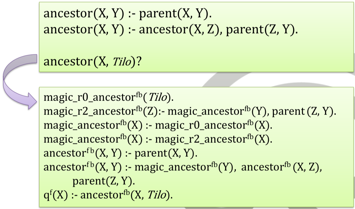
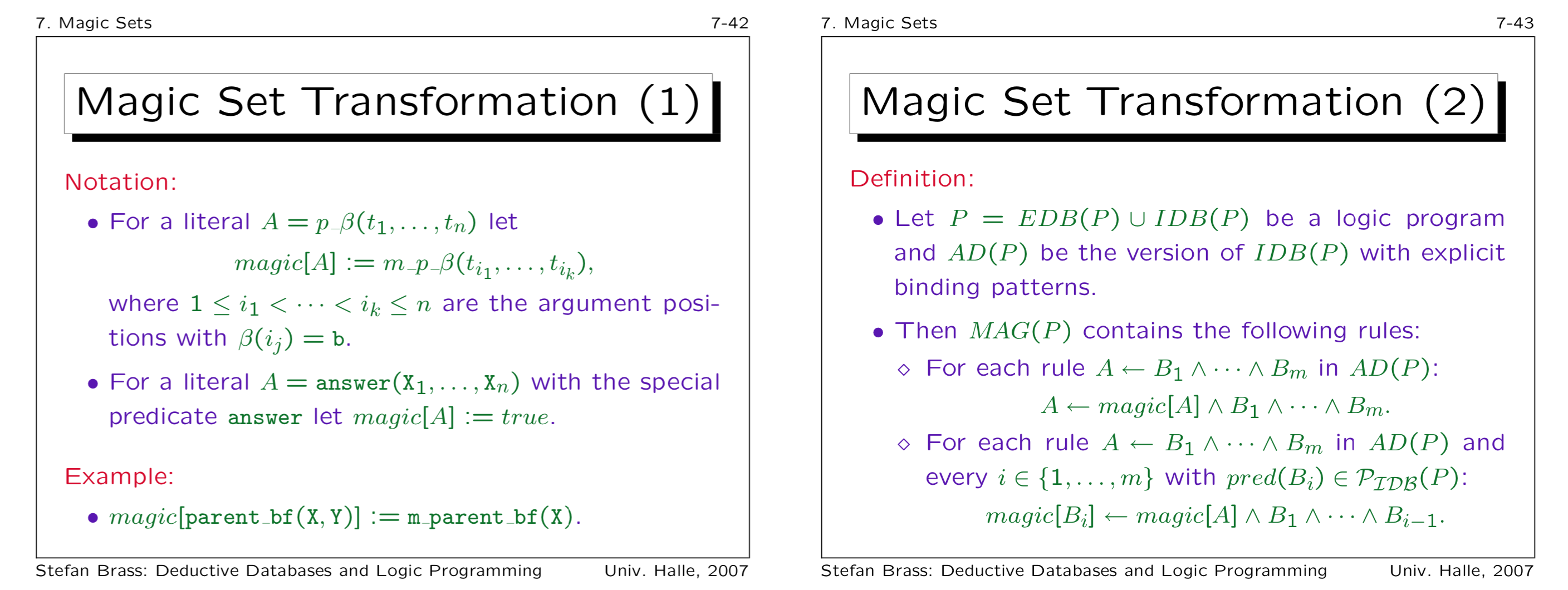 Source: Vorlesung aus Halle
5th Generation Project (D)
- Computer generations (1980s)
- 0th: Full mechanical computers using Punch cards (Harvard Mark 1, 1943)
- 1st: Pluggable vacuum cube (ENIAC, 1940)
- 2nd: Computers with transistors (after 1953)
- 3rd: Usage of integrated circuits (1964)
- 4th: Micro-processors (Intel 4004, 1971)
- Japan wanted to build the next generation
- Potential fields for a new generation:
- Inference computer technologies for knowledge processing
- Computer technologies to process large-scale databases and knowledge bases
- High performance workstations
- Distributed functional computer technologies
- Super-computers for scientific computing