Expert Systems
Basics
- Main application of AI in the 80s
- Expert System:
- System which can draw conclusions to support people in decision making
- Simulate a human expert
- Application
- Medical diagnosis (failure)
- Production/machine failure diagnosis (works well)
- Financial services (algo-trading, works well)
- User groups:
- End users:
- Group using the system for problem solving (e.g., doctors, mechanic)
- Domain experts:
- Group whose knowledge must be extracted (often, implicit knowledge)
- Knowledge Engineers:
- Bridge between domain expert and the developer
- Assist the domain expert by representing the knowledge
- End users:
- Construction:
- Build the knowledge base:
- Extract knowledge
- Very hard due to implicit knowledge
- Choose a reasoning technique
- Design the explanation facility (very hard)
- Build the knowledge base:
- Reasoning techniques:
- Datalog/Prolog (no uncertainty)
- Probabilistic approach
- Heuristic approaches (e.g., MYCIN, certainty factors)
- Fuzzy approaches (possibility)
- Case-Based reasoning
- Different models:
- Strict reasoning (purely logical, Datalog)
- Probabilistic reasoning
- Absolute statement
- Probabilistic frequencies
- Requires huge statistical evaluation
- Certainty factors
- Relative statements
- No (absolute) statistics necessary
Architecture
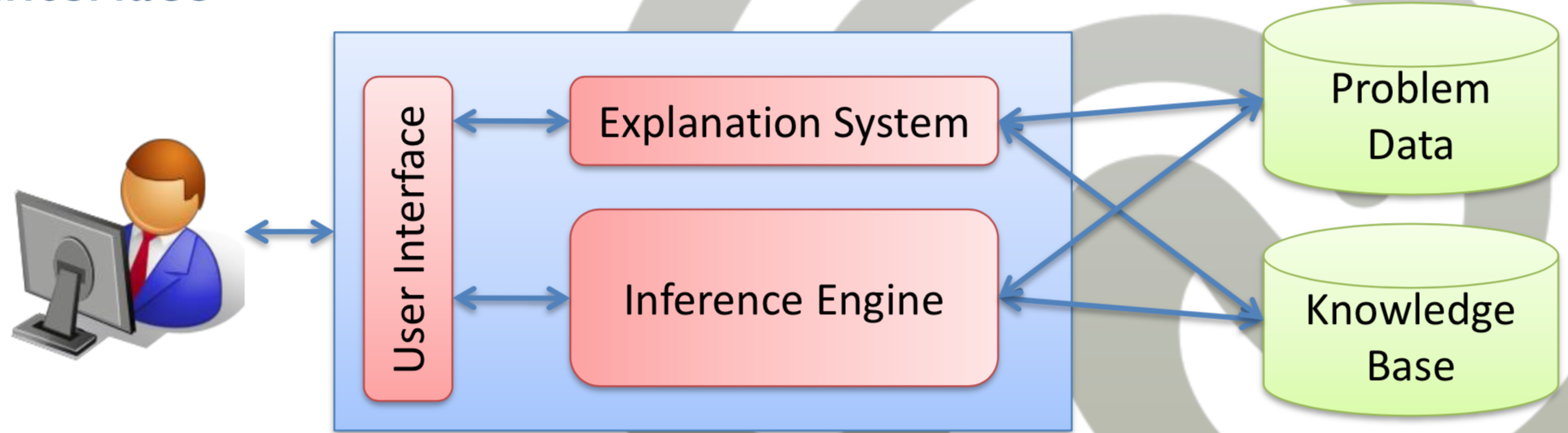
- User Interface
- Usually, question-response dialog
- Inference Engine
- Deduction system
- e.g., fuzzy reasoning, heuristics, case-based, …
- Responsible for efficiency, accuracy, …
- Explanation System
- Explain the answer to the user
- Knowledge Base
- Expert knowledge (also general)
- Set of rules and base facts
- Problem Data
- Specific problem data (e.g., expert system for cancer)
Uncertain Knowledge
- Uncertainty of deriving facts
- Rules can lead to multiple facts (which one is true?)
- e.g., headache –> hangover, headache –> flu
- Rules may only be valid in certain cases
- e.g., all birds fly; except penguins/ostiche
- Rules can lead to multiple facts (which one is true?)
- Sources of imperfect information
- Incomplete information (missing facts)
- Imprecise information (e.g., predicate young)
- Uncertain information (exceptions to rules, wrong defined predicates)
- Central question:
- How to deduce under uncertainty?
- i.e., probable and possible causes?
- Basic Idea:
- Assign Measure of validity to each rule/statement
- Propagate the measure through inference steps
- Measures:
- Probability truth values (use statistics, distributions)
- Possibility values (possibility distribution)
- Belief values (do not measure the probability of a cause, degree of belief)
- Requirement: Open World Assumption
- Makes reasoning more difficult
- Reasoning is not monotonic anymore (adding facts might refute/revise facts)
Non-Monotonic Reasoning (D)
- Statements considered true might be revised
- Knowledge is not monotonically growing
- e.g., if new knowledge is added
- Approaches are inspired by human reasoning
- Approaches:
- Default Logic
- Predicate circumscription
- Autoepistemic reasoning
Default Logic
- Raymond Reiter, 1980
- Idea:
- Statements, which are true by default
- Negative facts must be explicitly mentioned
- Default Theory \( T \):
- Two parts: \( D \) and \( W \)
- \( W \): Set of FOL rules known to be true (axioms)
- \( D \): Set of default rules
- \( \frac{\text{prerequisite : justifications}}{\text{conclusion}} \)
- Reasoning:
- If the prerequisite is true AND
- Each justification is consistent (non-contradictory) with the set of axioms/current beliefs THEN
- Believe that the conclusion is true
- e.g., \( \frac{bird(X):fly(X)}{fly(X)} \): As long as no bird \( X \) is not flying, it flies
- Common assumption: Closed World Assumption
- Default Rule: \( \frac{\text{true : }\neg F}{\neg F} \)
- Semantics:
- Based on fixpoints
- Given: Set \( W \), initial theory \( T \)
- After the deduction of a fact, check the fact for consistency
- e.g., protect against rules which add inconsistent knowledge
- Extensions of \( T \): Deduced facts
- Non-deterministic (deduced theory depends on sequence of default rules)
- Entailment of a formula from a default theory
- Skeptical entailment:
- Formula is entailed if its entailed by all its extensions
- Credulous entailment:
- Formula in entailed if its entailed by at least one extensions
- Skeptical entailment:
Predicate Circumscription
- John McCarthy, 1978
- Idea:
- Use common conceptions (things are as expected, unless specified otherwise)
- State facts which are not true
- Use Circumscription
- If a predicate does not hold, mention it
- Similar: Add \( \neg\text{abnormal}(X) \) to all rules
- Circumscription tries to derive minimal models
- Problem: Disjunctive information
Autoepistemic Logic
- Moore, 1985
- Idea:
- Express not only facts
- Express knowledge and lack of knowledge about facts
- Formalize non-monotonicity using the belief operator \( B \)
- Belief operator \( B(\cdot) \)
- Formula \( F \)
- \( \neg B(F) \): Do not believe formula \( F \)
- Axioms:
- All propositional tautologies are axioms
- If we believe in \( C(X)\leftarrow A(X). \)
- Inference rule: Modus ponens
- e.g., \( B(bird(X))\land\neg B(\neg fly(X))\rightarrow fly(X) \)
- Belief theory \( T \) describes the knowledge base
- We either believe or not believe a fact in the knowledge base
- A belief model must be consistent
Probabilistic Reasoning
Probability Theory
- Probability theory:
- Express belief/knowledge that a certain event occurred/will occur
- Two interpretations:
- Frequentist view:
- Probability is relative frequency of an event in a long running random experiment
- Bayesian view:
- Probability can be assigned to any event
- Probability: Degree of belief
- Frequentist view:
- Definition:
- Event \( A \)
- \( P(A)\in [0,1] \)
- \( P(\neg A) = 1-P(A) \)
- Statistical independence: \( P(A\land B)=P(A)\cdot P(B) \)
- Conditional probability: \( P(A\mid B) \)
- Bayes Theorem: \( P(A\mid B)=\frac{P(A\land B)}{P(B)}=\frac{P(B\mid A)P(A)}{P(B)} \)
- Probabilistic rules:
- \( B\leftarrow^{P(B\mid A)} A \)
- \( B\text{ :- }^{P(B\mid A)} A \)
Reasoning
- Goal: Combine facts/use rules (deductive chain)
- \( R(X)\leftarrow^{0.6} Q(X). \)
- \( S(X)\leftarrow^{0.9} R(X). \)
- \( S(X)\leftarrow^{0.54} R(X). \) (wrong)
- Problem:
- Naive approach of assuming statistical independence breaks
- Solution: Assume any relationship
- Chaining rule:
- Provide facts having a certain interval of confidence
- Non-monotonism: Adjusting intervals is revision
Confidence
- Possible relationships between events \( A \) and \( B \):
- Independence
- \( A\cap B=\emptyset \)
- \( P(A\land B)=P(A)P(B) \)
- Mutually exclusive
- \( A\iff \neg B \)
- \( P(A\land B)=0 \)
- Implication
- \( A\Rightarrow B \)
- \( P(A\land B)=P(A) \)
- No quantifiable relationship
- Boole: Provide an interval containing \( P(A\land B) \)
- \( \max(0,P(A)+P(B)-1)\leq P(A\land B)\leq \min(P(A), P(B)) \)
- Left side: Independence of events
- Right side: Implication
- Boundaries are called T-Norms
- Minimum T-Norm (Gödel T-Norm): \( \min(P(A), P(B)) \)
- Lukasiewicz T-Norm: \( \max(0,P(A)+P(B)-1) \)
- More cases (negative correlation, …)
- Independence
- Use intervals for \( P(A), P(B) \)
- Only possible case, since we have no information
- Confidence intervals:
- \( A\leftarrow^{(x_1, x_2)}B\iff 0\leq x_1\leq P(A\mid B)\leq x_2\leq 1 \)
- \( x_1=x_2:A\leftarrow^{x_1}B \)
- \( B\leftarrow^{(y_1, y_2)}A \)
- Converse: \( A_{(y_1, y_2)}\leftrightarrow^{(x_1,x_2)}B \)
Rule Types
- Causal rule:
- Relate known cause to its effect
- \( A \) cause for \( B \): \( B\leftarrow^{~1.0} A \)
- Deduction
- Usually have high probability
- e.g., \( groundIsWet\leftarrow^{1.0}sprinklerIsOn \)
- Diagnostic rule:
- Relate observed effect to its cause
- \( B\leftarrow^{<<1.0}A \)
- Abduction
- Usually have lower probabilities
- e.g., \( sprinklerIsOn\leftarrow^{0.2}groundIsWet \)
- Syntactic difference between the rules
- Strength of belief (high vs. low probabilities)
- Differentiation is done in big data (by correlation coefficient)
Chaining Rule
- Important:
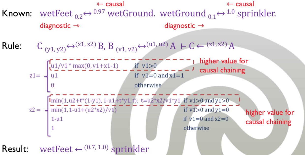
- Either use causal or diagnostic rules for deduction
- Otherwise, deduction is false
- Bi-directional rule:
- Combine causal and diagnostic rule
- \( A_x\leftrightarrow^y B \)
- e.g., \( sprinklerIsOn_{1.0}\leftrightarrow^{0.2}groundIsWet \)
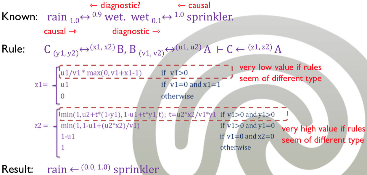
- Problem: Mixing two types does not work
- Example:
- \( groundIsWet\leftarrow^{1.0}sprinklerOn \) (causal)
- \( rain\leftarrow^{0.8}groundIsWet \) (diagnostic)
- \( rain\leftarrow^{0.8}sprinklerOn \) (wrong conclusion)
- Idea: Protect against mixing the rules
- Dampening function based on difference of probabilities
- Example:
- T-Norm Chaining rule:
- \( C_{(cb_1,cb_2)}\leftrightarrow^{(bc_1,bc_2)}B, B_{(ba_1,ba_2)}\leftrightarrow^{(ab_1,ab_2)} A\vdash C\leftarrow^{(ac_1,ac_2)}A \)
- \( ac_1 \):
- IF \( ba_1>0 \): \( \frac{ab_1}{ba_1}\cdot \max(0, ba_1+bc_1-1) \) (dampening)
- IF \( ba_1=0 \) and \( bc_1=1 \): \( ab_1 \)
- IF otherwise: \( 0 \)
- \( ac_2 \):
- IF \( ba_1>0 \) and \( cb_1>0 \): \( \min(1, ab_2+t(1-cb_1), 1-ab_1+t\cdot cb_1, t) \) with \( t=\frac{ab_2 bc_2}{ba_1 cb_1} \) (dampening)
- IF \( ba_1>0 \) and \( cb_1=0 \): \( \min(1, 1-ab_1+(ab_2 bc_2)/ba_1) \)
- IF \( ba_1=0 \) and \( bc_2=0 \): \( 1-ab_1 \)
- IF otherwise: \( 1 \)
- The interval only gets larger
- Deductive calculus
- Can prove the chaining rule (is correct)
- Rule is not very intuitive
- T-Norms apply worst-case estimation
- Deduction with Uncertain Knowledge (DUK calculus)
Example
 .
.
Belief Networks
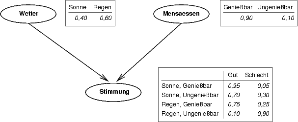
- Bayesian Belief Network
- by Judea Pearl, 1985
- Represent a set of random variables and their conditional probabilities
- Explicitly model independence relationships
- Directed acyclic graph
- Node: Random variable
- Annotated with conditional probabilities
- Root node:
- Assigned a prior probability
- Child node:
- Assigned conditional probability tables
- Edge: Direct (causal) influence between variables
- Missing edge: Conditional independence
- Node: Random variable
- Local Markov property
- Semantics of Bayesian Belief Network
- Full joint distribution is product of local conditional distributions
- Variable only depends on its parents
- \( P(X_1,\ldots,X_n)=\Pi_{1\leq i\leq n} P(X_i\mid parents(X_i)) \)
- These probabilities are available in the network
- Inference
- Beliefs are propagated
- \( P(H|X_1,\ldots,X_n) \)
- \( H \): Hypothesis
- i.e., use Bayes Theorem
- Inference is done by conditioning
 .
.
Heuristic Reasoning
MYCIN
- 1970, Stanford
- Medical expert system for infections
- ca. 600 rules (supporting uncertainty)
- Never used in practice (too unpractical)
- Legal and ethical issues (e.g., mistakes)
Design
- Uncertain reasoning
- No complete and no precise information in medicine
- Problem: No real distinction between doubt, missing knowledge or absence of belief
- Idea: Use Certainty factors (do not model measure of belief/disbelief)
Heuristic System
- Contains Rules (only confirming/disconfirming rules with certainty factors)
- Patient provides set of facts (e.g., age, general condition)
- Backward-chaining approach
- Generate proofs for most likely rules
- Request missing information from the user
- Provide all possible deductions with certainty factors
- Then, explain answers using the proof trees
Example Rule
IF the organism 1) stains grampos 2) has coccus shape 3) grows in chainsTHEN there is a suggestive evidence of 0.7 that it is streptococcus- The
0.7is the belief of the expert
Certainty Factor Model
- Invented in MYCIN
- Idea:
- Measure the relative change of belief of a hypothesis given an observation
- e.g., at first, believe in everything; then, change the belief
- Based on measure of belief and disbelief
- Independent
- e.g., increasing belief does not decrease disbelief
- \( CF(h\mid E)>0 \): Fact \( E \) confirms hypothesis
- \( MB \) and \( MD \) can be derived from \( CF \)
- \( MB(x)=\begin{cases}0 &\text{if } CF(x)<0 \\CF(x) &\text{otherwise}\end{cases} \)
- \( MD(x)=\begin{cases}-CF(x) &\text{if } CF(x)<0 \\0 &\text{otherwise}\end{cases} \)
- i.e., if the system only uses certainty factors
- e.g., MYCIN only uses certainty factors
Definitions
- Measure of belief
- For hypothesis \( h \) given observation \( E \)
- \( MB(h\mid E)=x \)
- Under evidence \( E \) the belief that \( h \) is true increases by \( x \)
- Number can not be computed, must be given
- e.g., \( MB(fly(X)|isBird(X))=0.8 \)
- Measure of disbelief
- For hypothesis \( h \) given observation \( E \)
- \( MD(h\mid E)=x \)
- Under evidence \( E \) the disbelief that \( h \) is true increases by \( x \)
- Number can not be computed, must be given
- e.g., \( MD(fly(X)|isBiggerThan(X, 2m))=0.8 \)
- Certainty Factor
- \( CF(h\mid E)=MB(h\mid E)-MD(h\mid E) \)
- \( CF\in [-1,1] \)
- Describe the change of belief when a given fact/observation is known
- \( CF>1 \): Belief increases (confirm)
- \( CF<1 \): Disbelief increases (refute)
- Relative measure combining disbelief and disbelief
- \( CF(h|E)+CF(\neg h|E)\leq 1 \)
- i.e., evidence for hypothesis does not support the negation of the hypothesis
Relation to Probability
- Rules for combination/chaining are required to deduce
- Assumption:
- The formal model matches the intended semantics of the informal definition (i.e., fuzzy concept of human belief)
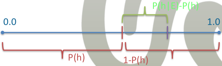
- Measure of Belief
- \( MB(h\mid E)=\begin{cases}\frac{\max(P(h\mid E), P(h))-P(h)}{1-P(h)} &\text{if } P(h)\neq 1 \\1 &\text{otherwise}\end{cases} \)
- \( MB(h\mid E)=0 \) if \( P(h\mid E)<P(h) \)
- Measure of Disbelief:
- \( MD(h\mid E)=\begin{cases}\frac{P(h)-\min(P(h\mid E), P(h))}{P(h)} &\text{if } P(h)\neq 0 \\1 &\text{otherwise}\end{cases} \)
- Certainty Factor:
- \( CF(h\mid E)=\begin{cases}\frac{P(h\mid)-P(h)}{1-P(h)} &\text{if } P(h\mid E)\geq P(h),P(h)\neq 1 \\\frac{P(h\mid)-P(h)}{P(h)} &\text{if } P(h)\geq P(h\mid E),P(h)\neq 0\end{cases} \)
- Basis:
- Definitions rely on the a-priori probabilities and conditional probabilities
- Must be given from expert (subjective measure)
- User-provided CF is a proxy for the real probabilities
Reasoning
IF a THEN h WITH CF(h|a)- Confirming rules: Positive CF
- Disconfirming rules: Negative CF
- Approaches:
- Rule Chaining
- Parallel Combination
Rule Chaining
IF e THEN a WITH CF(a|e)IF a THEN h WITH CF(h|a)- Result:
IF e THEN h WITH CF(h|e)
- Compute
CF(h|e):- \( CF(h|e)=MB(h|e)-MD(h|e) \)
- \( MB(h|e)=MB(h|a)\cdot \max(0, CF(a|e)) \)
- \( MD(h|e)=MD(h|a)\cdot \min(0, CF(a|e)) \)
Parallel Combination
IF e1 THEN h WITH CF(a|e1)IF e2 THEN h WITH CF(a|e2)
- Result:
IF e1, e2 THEN h WITH CF(a|e1,e2) - Combine multiple rules for the same hypothesis
- Compute the belief and disbelief values independently
- \( MB(h|e_1,e_2)=\begin{cases}0 &\text{if } MD(h\mid e_1,e_2)=1\\MB(h|e_1)+MB(h|e_2)-MB(h|e_1)MB(h|e_2)&\text{otherwise}\end{cases} \)
- \( MD(h|e_1,e_2)=\begin{cases}0 &\text{if } MB(h\mid e_1,e_2)=1\\MD(h|e_1)+MD(h|e_2)-MD(h|e_1)MD(h|e_2)&\text{otherwise}\end{cases} \)
- Combine to the certainty factor
CF(a|e1,e2)
Fuzzy Reasoning
- Idea: Model vagueness of information/language
- Fuzzy set theory (Zadeh, 1965)
- Express degree of possibility (probability uses crisp set membership)
- Focus: Possibility
Fuzzy Set Theory
- Universe \( \Omega \)
- Set membership function \( \mu_A:\Omega\rightarrow[0,1] \)
- e.g., degree that \( \omega\in\Omega \) is in the fuzzy set \( A \)
- \( (\mu_1\cap\mu_2)(\omega)=\min(\mu_1(\omega), \mu_2(\omega)) \)
- \( (\mu_1\cup\mu_2)(\omega)=\max(\mu_1(\omega), \mu_2(\omega)) \)
- \( (\neg\mu)(\omega)=1-\mu(\omega) \)
- Some characteristics of Boolean Algebra
Possibility Distribution
- Possibility theory (Zadeh, 1978)
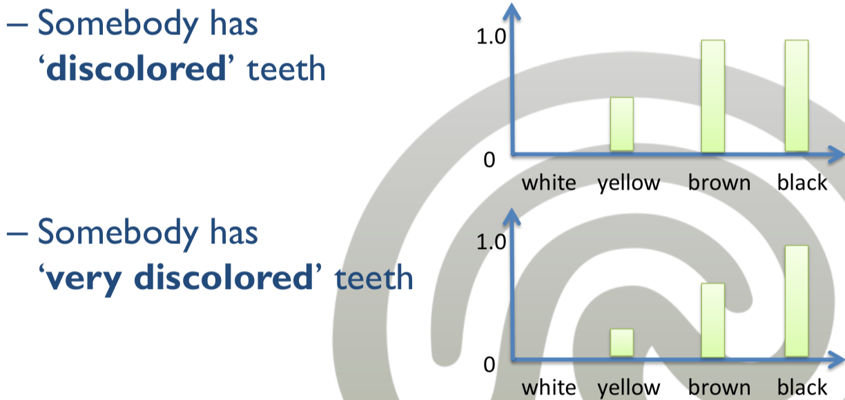
- Depend on a possibility for a certain case
- Possibility depends on estimations
- Possibility is an upper limit for probability
- Example:
- \( P(\text{teeth}=\text{discolored}, \text{Color}=\text{white})=0 \)
- \( P(\text{teeth}=\text{discolored}, \text{Color}=\text{yellow})=0.3 \)
Reasoning
Definition Hedge:
- Mapping between natural language and mathematical operations
- Example:
- Fact: Tom has yellow teeth.
- Rule: If a person has very discolored teeth, it is cavities.
- hedge very is defined as \( \mu_\text{very}(\omega)=(\mu(\omega))^2 \)
- \( \mu_\text{stained}(\text{Tom})=0.8 \)
- \( \mu_\text{very\_stained}(\text{Tom})=0.64 \)
- Other: very, few, more, less, rather, sort of
Task:
- Given fuzzy facts, deduce new fuzzy facts
- Match premise of rules and fuzzy facts
- i.e., fact X is A’
- \( A' \) may be a hedge of \( A \)
- Rule X is A, then Y is B
- Find relation between A and A’
- Result: Use possibility distributions
Goal: Link possibility to truth value of the conclusions
Combine two (or more) facts
- Aggregate facts (e.g., \( \min, \max,\ldots \))
- e.g., clipping or scaling
- Aggregate possibility distribution (e.g., conjunction)
Done by the inference process
Inference Process
- Mamdani, 1975
- Steps:
- Fuzzification
- Inference
- Composition
- Defuzzification
Fuzzification
- Initialize the membership degrees for input variables
- Given by the membership function
- Determine the degree of truth for each rule premise
- Tilo: Different possibilities of different premises
- Example:
- Input:
- Tom’s teeth have yellow stains
teeth_color(yellow) := color_yellow
- Fuzzy sets in the database:
slightly_discolored,discolored,very_discolored
- Determine:
- \( \mu_{slightly\_discolored}(color\_yellow) = 0.3 \)
- \( \mu_{discolored}(color\_yellow) = 0.5 \)
- \( \mu_{very\_discolored}(color\_yellow) = 0.4 \)
- Input:
Inference
- Steps:
- Apply inputs to fuzzy rule
- Calculate degrees of the conclusion
- Apply the truth value of each premise of each rule (given by fuzzification) to compute the conclusion
- Methods:
- Clipping: Take the value of the premises as lower bound (e.g., if the premise is sure to 30%, the conclusion is sure to 30%)
- Scaling: Multiplying all membership degrees of multiple premises (e.g., first premise has 0.3 and second premise has 0.6, the conclusion has a fuzzy value of 0.18)
- Result:
- Fuzzy distribution over all possible rule conclusions/targets
- Example:
- Rules:
teeth_color=slightly_discolored --> cavities unlikelyteeth_color=discolored --> cavities possibleteeth_color=very_discolored --> cavities sure
- Distribution for
cavities:cavities(unlikely) = 0.3cavities(possible) = 0.5cavities(sure) = 0.4
- Rules:
Composition
- Aggregation
- Same conclusion can be produced by multiple rules
- Outputs of all rules are unified
- Example:
- Rules:
teeth_color=discolored --> cavities possible
xray=dots --> cavities possible
- Distribution for
cavities:- Result of 1:
cavities(possible) = 0.3 - Result of 2:
cavities(possible) = 0.7
- Result of 1:
- Result:
cavities(possible) = {0.3, 0.7}
- Rules:
Defuzzification
- Combine multiple membership degrees for a given conclusion
- Most common: Centroid technique
- Split set into two classes (center of gravity)
- Example:
- Result of composition:
cavities(unlikely) = {0.1, 0.3}cavities(sure) = {0.3, 0.7}
- Defuzzification:
cavities = 0.35
- Result of composition:
Example
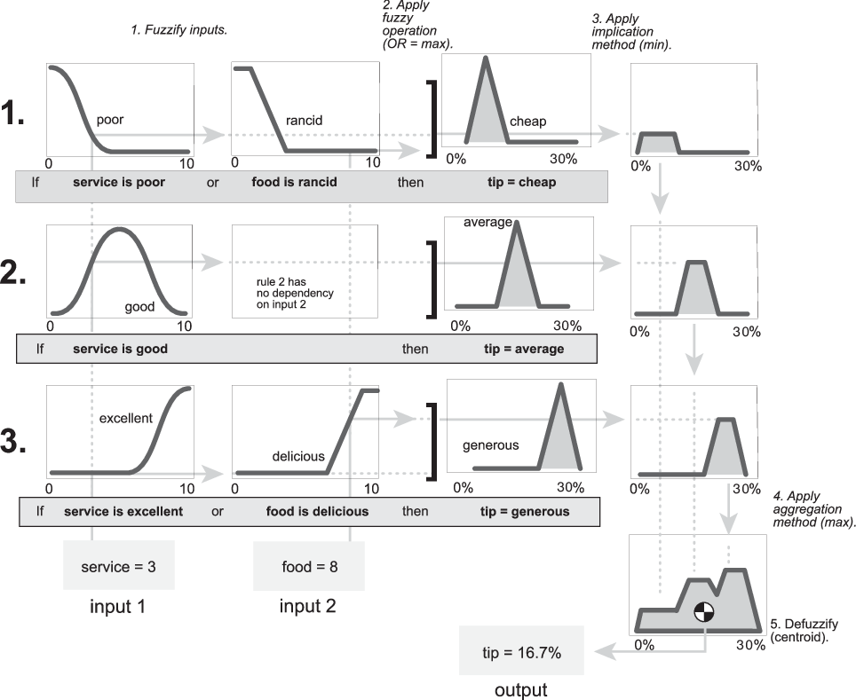
- Variables:
service,food - Target:
tip - Rules:
service=bad AND food=bad THEN tip=cheapservice=good THEN tip=averageservice=excellent AND food=delicious THEN tip=large
- Input:
service=3food=8
- Steps:
- Fuzzification:
- Rule 1: service(bad) = 0.3, food(bad)=0
- Rule 2: service(good) = 0.7
- Rule 3: service(excellent) = 0, food(delicios)=0.8
- Inference (MAX):
- Rule 1: tip(cheap) = 0.3
- Rule 2: tip(average) = 0.7
- Rule 3: tip(large) = 0.8
- Composition:
- see picture (step 4)
- Defuzzification:
- Compute centroid: tip=16.7 %
- Fuzzification:
 .
.
Case-Based Reasoning (CBR)
- Idea: Solve problems by using previous experiences
- More a heuristic (than a formal process)
- Similar to case-based law systems/medical diagnosis
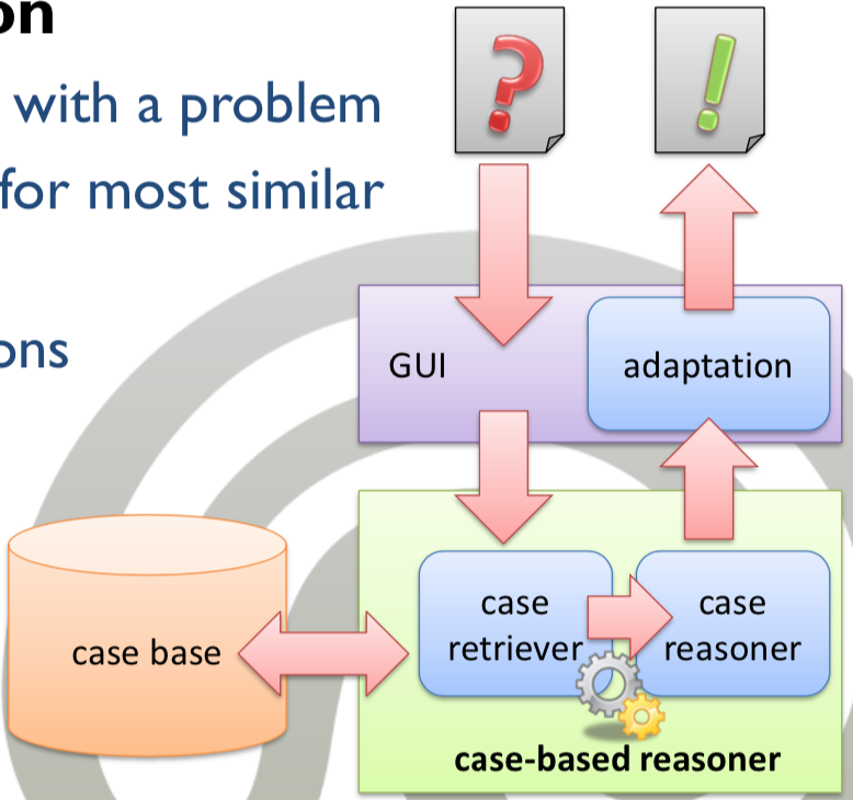
- Operation:
- Provide problem to system
- Search the case-base for similar problems
- Return solutions
- Case:
- Record of previous experience
- Properties:
- Problem specification
- Relevant attributes
- Applied solution
- Case-based vs. rule-based:
- Rule-based:
- Abstract knowledge (IF…THEN…)
- Acquired before the system can be used
- Case-based:
- System is continuous process
- Rule-based:
- When to use:
- Underlying model of the domain (CBR does not capture randomness)
- Exceptions/novel cases
- Re-occurring cases
- Significant benefit when adapting past solutions
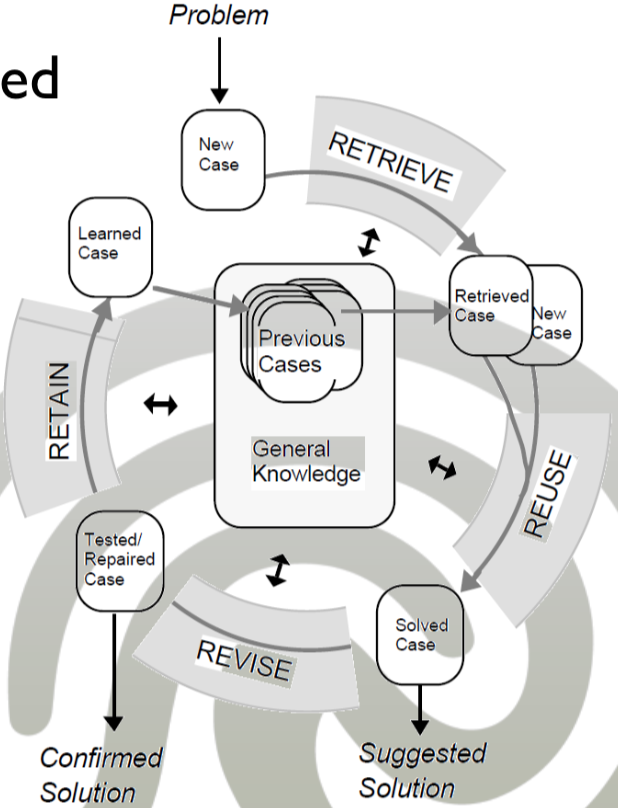
4-Phase-Model
- Aamodt/Plaza, 1994
- Phases:
- Retrieve: Retrieve similar cases (similar and not similar cases)
- Reuse: Map solution from retrieved case to target problem
- Revise: Test if solution fits (real-world or simulation)
- Retain: Store successfully adaption
Tasks
- Case Retrieval:
- Process of finding closes cases
- Approaches:
- Feature approach (can be indexed)
- Syntactic approach vs. semantic approach (Problem: similarity measure)
- Semi-automatic
- Case adaption:
- Translate retrieved solution to target problem
- Reuse base: Basic adaption
- Revise phase: Learning from failure
- Manual process
- Measure the degree of success
- Case-base maintenance:
- Part of the retain-phase
- Tradeoff performance vs. quality