Audio Retrieval¶

Basics of Audio¶

Origin: Audio, latin for I hear
Types of data:
- Music
- Spoken Text (e.g., Podcast, Speech)
- Noise (e.g., laughter, sounds of gears of cars, sound effects earcons)

Perception¶

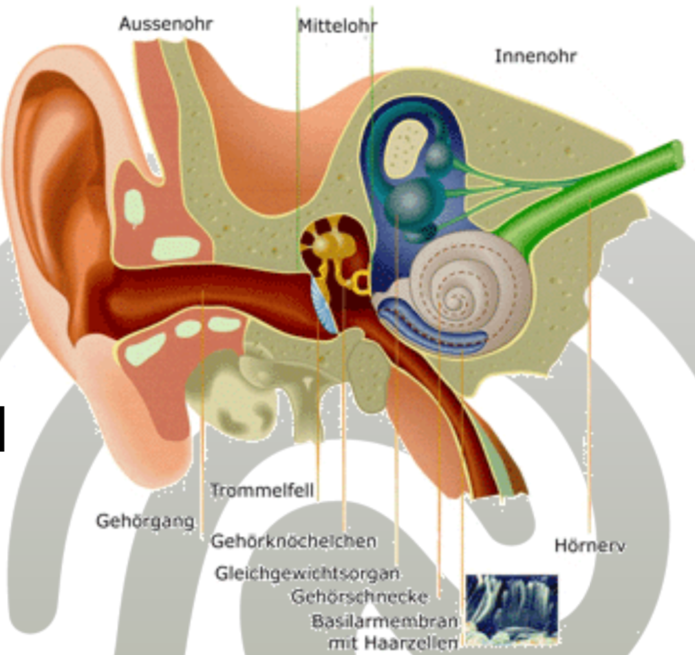
Information flow
- Pressure fluctuation in air (longitudinal wave)
- Eardrum (Trommelfell) vibrates
- Ear bones amplify + transmit vibration
- Hair cells in ear cochlea (Hörschnecke) are stimulated
- Neurons produce electrical impulse
Brain interprets two properties of sound
- Pitch (Tonhöhe)
- Volume (Lautstärke) measured in Dezibel

../_images/06-cochlea.png

Physics¶

Amplitude as volume
- Logarithmic perception
- Tenfold increase of Amplitude –> Double perceived loudness
- Usually measured in Dezibel (dB)
Frequency as pitch
- Hearing range: 20 Hz - 20 kHz
Audio signal is time-dependent

Sound Creation¶

Vibration generator:
- Instruments are Vibration generator
- Used to classify instruments
- e.g., String, Blow, Percussion
- Creates acoustic
Oscillator
- Used for synthetic sound creation
- Generates periodic voltage oscillations
- Speaker
  - Purpose: Transmit voltage change to membrane
  - Voltage change moves membrane
  - Membrane moves air
- Pitch: Higher voltage => Higher frequency
- Volume: Amplifier amplifies wave
- Sound modeled by ADSR envelope
ADSR envelope
- Curve describing the amplitude over time
- Influence loudness of sound over time (until key is released)
- Phases:
  - Attack:
    - Time to reach maximum amplitude
    - Speed of signal rise
    - Starts with key press
  - Decay:
    - Time in which the signal decreases to sustain
    - Starts immediately after end of attack phase
  - Sustain value:
    - Amplitude while the key is pressed
    - Starts after decay phase
  - Release:
    - Time in which the signal decreases to zero
    - Time in which sound is going on sounding

Digitalization¶

Task: Transform continuous wave into discrete representation

Sampling¶

Take current amplitude at regular intervals
Components
- Sampling rate:
  - Frequency of taking samples
  - e.g., CD 44.1 kHz, Phone 8 kHz
- Resolution:
  - Accuracy to record the values
  - e.g., 16 bit
Goal:
- Uniquely reconstruct the original oscillation
- Minimal but sufficient number of samples (to save memory)
Sampling theorem
- Nyquist, 1928
- Sampling rate must be at least twice as large as the highest occurring frequency in the signal
- \( f_{ny} \geq \frac{1}{2} \cdot f_{max} \)
Example CD
- Sampling rate: 44100 Hz
- Resolution: 16 bit
- 2 channels
- \( 44100 * 16 * 2 = 176400 \frac{B}{s} \approx 635 \frac{MB}{h} \)

Formats¶

Idea: Use compression to save space
Uncompressed formats
- AIFF: Apple Inter-opportunity File Format
- Wave
- IRCAM (*.snd): Institut de Recherche et Coordination Acoustique et Musique
- AU: Sun Audio
Reduction types
- Lossy
- Lossless
MIDI Format
- Musical Instrument Digital Interface
- Purpose: Transmission, recording, playing musical control information
- Statements are commands (e.g. from keyboard for synthesizer)
- No original sound
- Output via synthesizer

Lossless Reduction¶

Formats
- Free Lossless Audio Codec (FLAC): 50%-60% reduction
- Apple Lossless
- WavPack
Factors:
- Compression speed
- Compression rate (effectivity)

Lossy Reduction¶

Usually, based on simple transformations
- Modified Discrete Cosine Transformation (MDCT)
- Wavelets
Encoding: Transform wave into frequency sequences (sampling)
Decoding: Reconstruct original oscillation
Idea: Change data without changing subjective perception
- Omit very high/low frequencies (which can not be heard)
- Use other effects of psycho-acoustic model
  - Low tones after very loud tones
  - Extremely small frequency changes
Formats
- MPEG-1 Audio Layers (MP3)
  - Versions I, II, II
  - Cut un-hearable frequencies
  - Channel coupling (compress stereo by using the difference)
  - Huffman encoding for compression
- CD quality with 128 kb/s
- Advanced Audio Coding (AAC)
  - Industry-driven MP3 improvement
  - Used in TV-/radio, iTunes Store
  - Better quality compared to MP3
  - Support Multi-channel audio
- Ogg Vorbis
- WMA 9
Factors:
- Compression speed
- Compression rate
- Compressed audio quality (most important)

Audio Information In Databases¶

Audio information is mostly information transfer (e.g., speeches, recording of phone calls/conversations)
Storage
- Compressed audio files in (smart) BLOBs
- Metadata and feature vectors are stored for search functionality
- Additional information, e.g., transcription as text, musical notation, MIDI
Applications:
- Identification (audio as query)
  - e.g., Shazam (find title for music piece), Legal services (GEMA)
  - State of the art: Successful research
- Classification/similarity search (matching)
  - Find perceptional similar audio signals
  - e.g., similar songs, same quotation
  - Recommendation (e.g., similar songs)
  - Classification (e.g., rock, techno)
  - State of the art:
    - Manual annotations
    - Classification only works on small collections
    - Matching largely unresolved
- Phonetic synchronization
  - e.g., Speech to text, notes to audio
  - Retrieve text from speech (speech to text, text retrieval)
  - Follow audio scores
  - State of the art:
    - Tolerable error rates (language to text)

Basics¶

Metadata-based search
- Semantic metadata: Hard to generate (e.g., title, artist, speaker)
- File information: Automatically generated (e.g., time of recording, location, size, length)
- Problems:
  - Manual indexing is expensive
  - Incomplete/partial information
  - Subjective information (e.g., genre)
  - No query-by-example
Content-based search
- Naive: Compare sample-by-sample (not possible)
- Differentiate by (perceptual) characteristics
  - Low-level features (e.g. properties of sounds)
  - Logical/acoustic features (e.g., pitch, melody)
- Usually, audio is split into windows
Further reading:
- Music Lab
- Pitch and Frequency

Query-By-Example¶

Goal:
- Melody is central importance
- Use Query-By-Example (query the melody)
Limitation:
- We do not consider features like rhythm
Query inputs:
- Sample audio files
- Humming
- Whistling
- Singing
Major problems:
- Definition of melody (pitches, musical scales, variations, intervals, frequency jumps)
- Formulation of query
Idea: Use characteristic melody (not complete song)
- What is it?
- How to represent?
- How do queries look like?
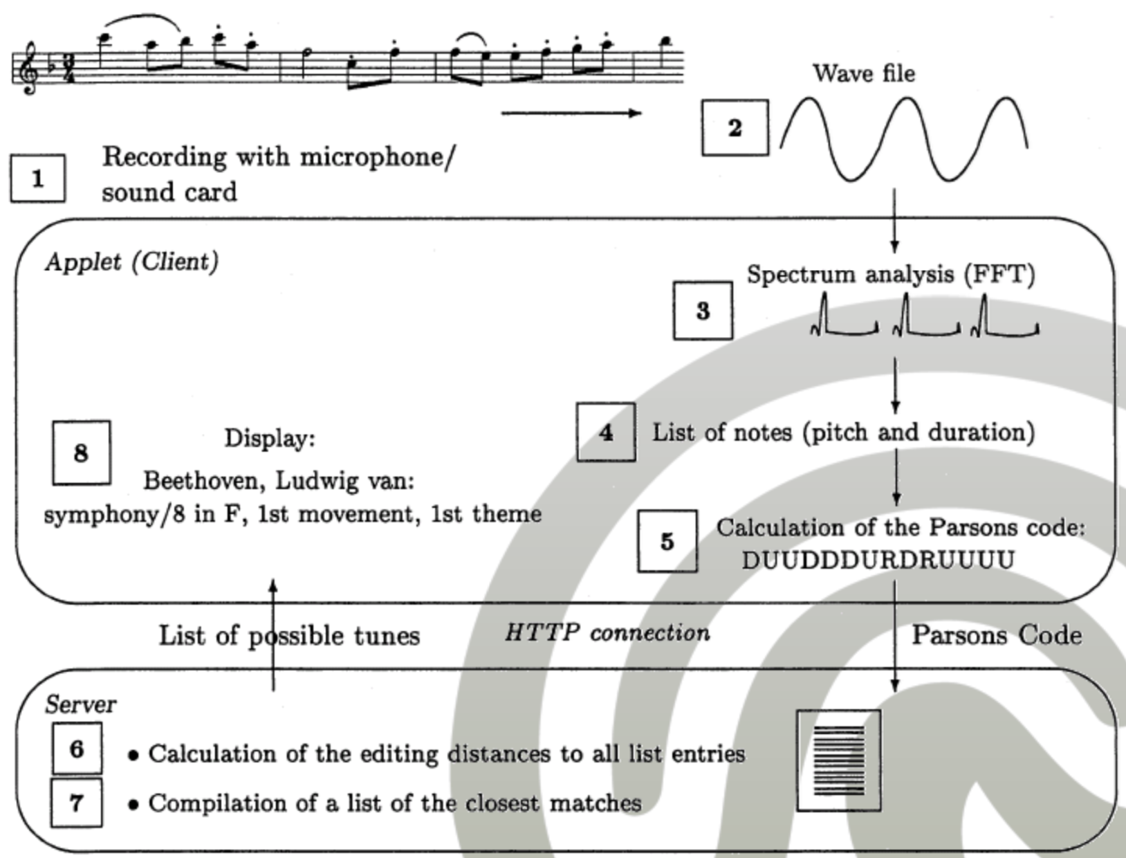
Model-based approach
1. Formulate query (humming, whistling, audio file)
2. Melody extraction (Fourier analysis, noise reduction, pitch tracking)
3. Encode melody (e.g., Parsons code, Differential code)
4. Similarity search in database
5. Return results

Architecture¶

../_images/08-arch.png

Input¶

Singing:
- Difficult (strong individuality of users)
Humming:
- Idea from Ghia et al., 1995
- Separate notes with sound for better detection
- e.g., ta
Whistling:
- Little individuality
- Good note separation
Virtual instrument:
- e.g., provide virtual piano
- Greenstone library, NZ

Melody Extraction¶

Sampling (of Digital Recording):
- Low sampling rate is sufficient (low quality of input)
- Requires noise reduction
- Group samples by overlapping (sliding window)
  - Frame size: 50 ms
  - Frames are half-overlapping
Conversion:
- Compute spectral sample (spectrum) of each frame
- e.g., Short-Time Fourier Transform (STFT)
- Pitch per spectrum (Volume: avg. amplitude)
- Mark as silent frame if volume too low
Find note boundaries:
- Note boundary marked by silent frames or frequency jumps
- Heuristics:
  - Between two frames with a frequency jump: Add new silent frame (e.g., 3 % ratio of two frequencies)
  - Between two frames with same frequency and a single frame with different frequency in between: Replace with neighboring frequency (called Smoothing)
  - Between silent frames the frequency varies: Replace with average frequency
- Connect the same pitches to notes:
  - Connect equal/same pitches between silent frames to one note with higher duration
  - Remove notes with a length below a threshold (this is Noise)
  - Remove all silent frames
Output: Melody with note pitch and duration

Spectrograms¶

Motivation:
- Time-domain doesn’t contain frequency components
- Frequency-domain doesn’t contain time of frequencies ocurring
- Solution: Combine time- and frequency domain
Computation:
- Perform Fourier Transform on time windows
3-dimensional diagram
- X-axis: Time
- Y-axis: Frequency
- Gray-value of pixel: Intensity of frequency at time
Can be used to analyze the regularity of occurring frequencies

Low-level Features¶

Acoustic features
- Describe signal by statistical properties of characteristic values (compare to image database)
- Use time-dependent vector function (instead of feature vector)
Measurements
- Time domain (amplitude vs. time)
- Frequency domain (intensity vs. frequency, e.g. Fourier transformation)
Notation: Signal consists of \( N \) points \( x_N \)

Time domain¶

Mean amplitude:
- \( \frac{1}{N} \sum_{i=1}^N |x_i| \)
- Fluctuation around zero (silence equals 0 amplitude)
Average Energy
- Average volume of signal
- \( \frac{1}{N} \sum_{i=1}^N x_i^2 \)
Zero-crossing rate
- Frequency of sign change
- \( \frac{1}{2N} \sum_{i=1}^{N-1} |sgn(x_{i+1}) - sgn(x_i)| \)
- Sometimes, the variance of the zero-crossing rate is used (audio is split in windows)
Silence ratio
- Also called Portion of silence
- Proportion of values belonging to period of complete silence
- Requirements:
  - Amplitude threshold (When is a sound silent?)
  - Number of consecutive measurements that are considered as silence period

Frequency Domain¶

Foundation: Fourier transform
- Decompose audio into frequency components with coefficients
- Frequency spectrum
- Coefficient: Its size represents the amount of energy per frequency (usually measure in decibels)
Bandwidth
- Interval/range of occurring frequencies
- \( f_{min}-f_{max} \)
- \( f_{min} \) is first frequency above silence-frequency (threshold)
- Use for classification: Bandwidth of music is greater than bandwidth of voice
Brightness
- Center-of-gravity/expected value of frequency distribution
Power distribution
- Also called ‌Energy distribution (distribution of the Fourier coefficients over the frequencies)
- This is no direct measure
- Other measures can be derived (such as brightness)
- ~~Calculate frequency bands with high/low energy~~
Harmony
- Harmony is a perceptional property describing the well-sounding of a melody
- Definition Fundamental frequency: Minimal (lowest) loud frequency
- Harmony is given if the dominant components of the spectrum (frequencies) are multiples of the fundamental frequency
- Harmony is continuous measure
Pitch
- Pitch is an perceptual property (Tonhöhe)
- Calculate from frequencies and amplitudes of peaks (e.g., using the Harmonic Product Spectrum, MLE, etc.)
- Pitch is not the fundamental frequency
- Pitch is related to frequencies (often used as approximation; not the same)

Classification¶

Goal: Differentiate between music and noise
Different audio classes have typical values for these features
- Features must differentiate enough
- e.g., speech, techno, classic, ambient, electronic)
Training:
- Use a perceptional model
- Compute a reference vector for each class
Classification:
- Classify based on the minimal distance (e.g., 1-NN)
Evaluation:
- Works good as coarse classification (speech vs. music)
- Works bad to classify musical pieces into genres

Approach Lu et al.¶

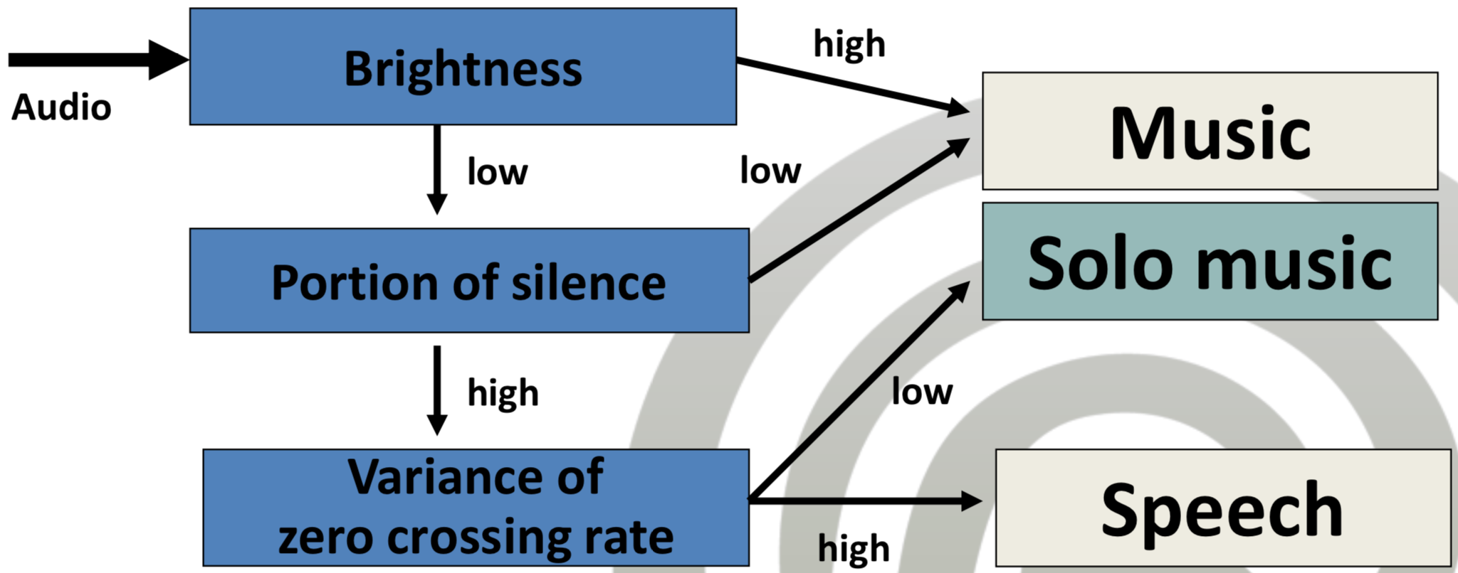
Lu/Hankinson (1998)
Use case: Distinguish between speech and music
Idea: Use complete signal
Combine these features:
- Bandwidth
  - Speech: 100 Hz - 7000 Hz
  - Music: 16 Hz - 20000 Hz
- Brightness
  - Speech: Low
  - Music: High
- Proportion of silence
  - Speech: Frequent
  - Music: Low (except solo instruments)
- Variance of zero-crossing rate
  - Speech: Characteristic structure in syllables (fluctuating zero-crossing rate)
  - Music: Consistent rhythm (rather constant zero-crossing rate)
Algorithm:
- Note: Estimates of low and high are collection-dependent (determine by training examples)

../_images/07-lu.png

Approach Wold et al.¶

Wold et al., 1996
Goal: Perceptional comparison of audio files
Idea:
- Divide audio signals in time slots
- e.g., due to different sounding slots in music
- Compute feature vector and statistical properties for each window
Feature vector:
- Compute statistical features over the four coefficients
- Compute statistics over (1) the windows and (2) the whole signal
- Coefficients:
  - Loudness
  - Brightness
  - Bandwidth
  - Pitch
- Statistical features:
  - Expected value (average value)
  - Variance (mean square deviation)
  - Autocorrelation (self-similarity)
- Results in a 12-dimensional feature vector
Approach implemented in:
- DB2 AIV Extender
- Oracle multimedia

../_images/07-windows.png

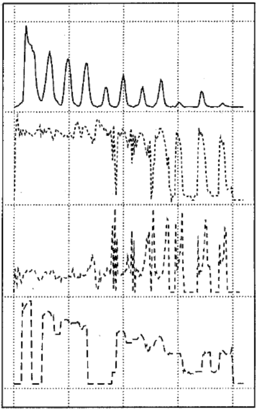
Statistical Characteristics¶

Loudness / Perceived volume
- Root mean square (RMS) of amplitude values (in dB)
- Root mean square:
  - \( RMS=\sqrt{\frac{1}{n} \sum_{i=1}^n x_i^2} \)
  - Weight higher values higher than lower
- Other methods: Take different perception of frequencies into account (e.g., lower 50 Hz, above 20 kHz)
Brightness / Perceived brightness
- Definition: Expected value of Fourier spectrum
- Logarithmic scale
- Describes the amount of high frequencies in signal
Bandwidth / Frequency bandwidth
- Variance of the signal:
  - Weighted average of differences of Fourier coefficients of center-of-gravity (expected value) of spectrum
  - Weights: Amplitudes
Pitch
- Perceived pitch (pitch is usually different from frequency)
- Calculate: Frequencies and amplitudes of peaks in each interval (by pitch tracking)
- Pitch tracking is difficult (simply, approximate by fundamental frequency)

Static Classification¶

Training:
- Input: Group of sounds of one class
- Compute the mean vector \( \mu=\frac{1}{N}\sum_{i=1}^N x_i \)
- Compute covariance matrix \( R=\frac{1}{N}\sum (x_i-\mu)(x_i-\mu)^T \)
Classification:
- New item \( x \)
- Compute Mahalanobis distance to each class, i.e., 1-NN classification
- \( D=\sqrt{(x-\mu)^T R^{-1}(x-\mu)} \)
- Compute probability of correct classification:
  - \( L=e^{-\frac{D^2}{2}} \)
  - Higher distance –> lower probability of correctness
- Order the distances by these values and select the one with highest probability

../_images/07-example-class.png

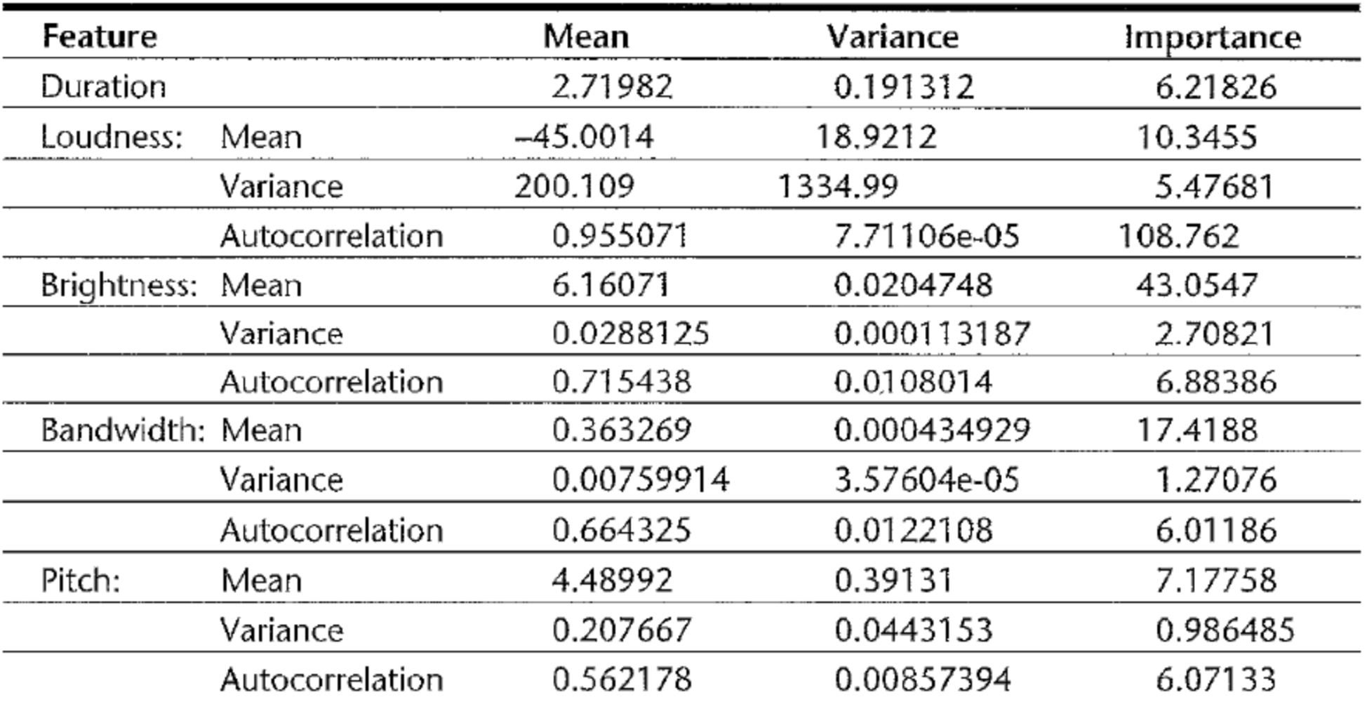
Evaluation¶

Works quite well for short audio
- e.g., sounds, speech
- Differentiate between speech and music/laughter and music
Advantages:
- Parameters statically represent human perception
- Easy to use
- Easy to index
- Query-by-example
Disadvantage:
- Statistical values are bad for musical pieces
- Bad to classify musical pieces
- Pitch determination does not work well

Melody Recognition¶

Goal: Detect melody of music/recognize notes from signal (trivial for MIDI file)
Definition Melody:
- Sequence of musical notes (sequence of differences)
Requirements for querying:
- Query-by-Humming
- Invariant under pitch shift (soprano/bass)
- Invariant under time shift
- Invariant under slight variations (users are not singers)
Problems:
- Different instruments overlap
- Detecting the dominant pitch is difficult due to interference
- Pitch is not the fundamental frequency
- Pitch has something to do the the frequencies
- Human perception differs from physical measurements
Harmonics:
- One main oscillation, several multiples overtones

Difference Limen¶

Definition Difference Limen:
- Also called ‌just-noticeable difference
- Smallest change in frequency that can be reliably perceived
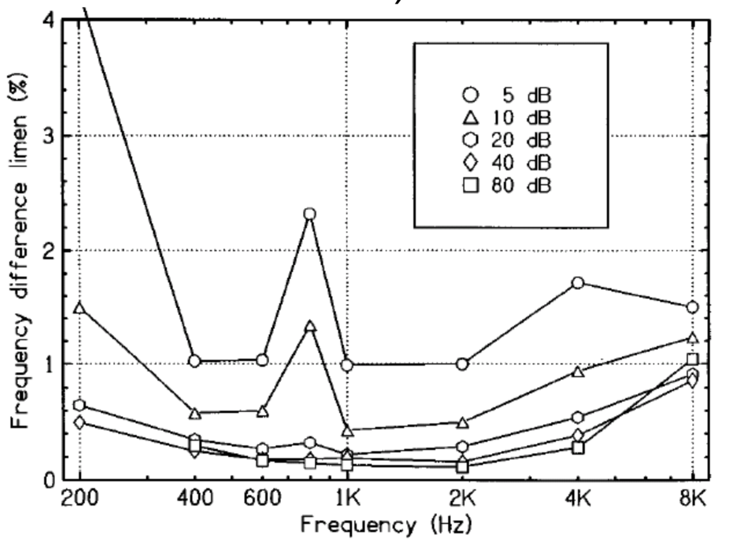
- Depends on pitch, duration and volume
Psychological Tests
- ‌Jesteadt et al., 1977
- They created perceptual scale of pitches
- Play two tones (each 500 ms) with small change
- Results in a psychometric function
Normally difference limen: 0.2 %
Influences:
- Frequency: Not uniform (possibly logarithmic)
- Duration: increasing from 0 - 100 ms, then constant
- Volume: increasing from 5 - 40 dB, then constant

../_images/07-limen.png

Pitch Determination¶

Definition Pitch (Tonhöhe):
- ANSI, 1994
- Perceptual property to order sounds from low to high
- Depends on mainly on frequency, pressure and waveform
- Distinguish pitch from timbre (Klangfarbe)
- ~~Pitch is feature of frequency at particular time (==What does that mean???==)~~

Biological Models¶

Cochlea:
- Spiral with little hairs which are connected to neurons
- Apex: Center of the spiral
- Oval window: Entrance of spiral
- Basilar membrane: Membrane inside the Cochlea covered by the hairs
- Different frequencies are perceived at different places inside the Cochlea
- Frequencies are perceived from high to low from the oval window to the apex
- Temporal synchronization of neurons: Neurons fire randomly
Problem of these models:
- Recognize only pitches of individual sounds
- Complex tones are more complicated
  - Multiple frequencies lead to multiple triggered locations
  - Multiple frequencies lead to interfering synchronization patterns

Location-dependent Model¶

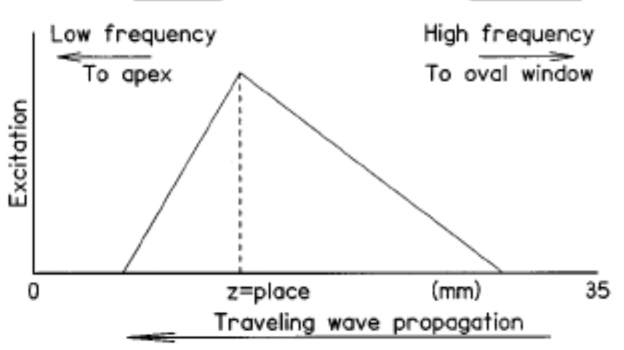
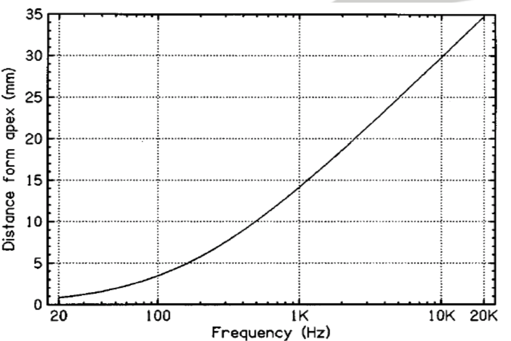
Idea: Detect pitch by perception location inside the cochlea
Lower frequencies travel farther inside the cochlea
Use function of excitation (distance from apex, in mm) as representation for pitch
Greenwood, 1990:
- \( z = 7.24 \cdot \ln (1+f/165) \) (Greenwood et al., 1990)

../_images/07-location.png ../_images/07-apex.png

Time-dependent Model¶

Sound coding not only location-dependent, also temporal synchronization of neurons are important
Refraction time: Cooldown of a neuron that has fired
Neuron behavior: Neuron fires spontaneously and randomly
Sound leads to synchronous fire rate which is detected by the brain
Auto-correlation of this pattern (e.g., ACF and AMDF)

Pitch Tracking Algorithms¶

Use time-dependent model
- Pitch of note can be perceived constant with and without fundamental frequency
- Removing fundamental frequency would change location in location-dependent model
- Synchrony of wave remains the same because of the harmonics
Hearing
- Complex sounds are analyzed in frequency bands
- Idea:
  - Match sound against harmonic templates to detect pitch (Goldstein, 1973)
  - e.g., Harmonic Product Spectrum, MLE
- Pitch is synthesized by hearing
  - Two distinct units on the ears are perceived as pitch
  - Non-occurring frequency can be “heard”
- Ambient noise can influence perception (the brain is tricked
Window size: twice as long as estimated period of wave
Requirements for algorithms:
- Frequencies must be on the range of a semitone around its correct octave
- Instruments must have well-defined harmonies (e.g., Cello, Piano)
- Real-time conversion of the signal (for real-time applications, e.g., Shazam)

Harmonic Product Spectrum¶

Schroeder, 1968 / Noll, 1969
Idea:
- Use frequency domain
- Analyze certain frequency bands (application-dependent)
- Analyze all frequencies from this band for harmonics
- HPS of a frequency provides an indicator of the “harmonic-ness”
Formally
- \( R \): Number of harmonics (e.g., 5)
- \( X(w) \): Strength of frequency \( w \) in current time window
- \( Y(w) \): Product spectrum of frequency \( w \)
- \( \hat{Y} \): Detected Pitch
- \( Y(w) = \Pi_{r=1}^R |X(wr)| \)
- \( \hat{Y} = \arg\max_{w_i} Y(w_i) \)
Advantage:
- Simple/robust
Problems:
- Noise below 50 Hz
- Octave errors:
  - Overtones are detected as pitch as well
  - Pitch may be recognized one or multiple octaves too high
- Solution: Rule-based
  - If closest amplitude under the pitch candidate has half its frequency and an amplitude over a certain threshold, select this as pitch

Maximum Likelihood Estimator¶

Noll, 1969
Goal:
- Detect pitch and
- Remove artifacts (false high frequencies)
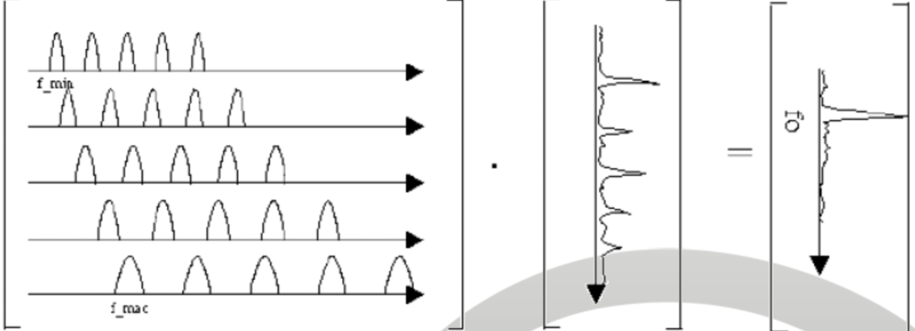
Idea:
- Use frequency domain
- Convolute with an ideal specter, i.e., chain of pulses (convolution is done using a dampening function, to be more robust)
- Minimize error for the frequencies (minimal error corresponds to the pitch)
Formal
- \( f \): Original signal
- Ideal specter
  - \( W \): Dampening function (to remove artifacts)
  - \( X \): Chain of pulses for the harmonics
  - \( Y_w \) ideal specter for frequency \( w \)
  - \( Y_w=X(w)*W(w) \) (convolute pulses with dampening function)
- Pitch (to detect) \( \hat{Y} \)
- \( \tilde{Y}_w = f*Y_w \): Convoluted signal for frequency \( w \)
Error
- Use discrete functions (vectors)
- Goal: Minimize error between ideal specter and convoluted signal (Maximum likelihood method)
- \( E(w) = ||Y_w-\tilde{Y}_w||^2 = ||Y_w||^2 + ||\tilde{Y}_w||^2 - 2Y_w\tilde{Y}_w^T \)
- \( ||Y_w||^2 \), \( ||\tilde{Y}_w||^2 \) remain constant
- \( \hat{Y} = \min_w E(w) = \max_w Y_w\tilde{Y}_w^T \)
  - Vector of different \( Y_w \) and the original signal \( f \)
  - Take maximal component of resulting vector
Good results if ideal specters are close to real specters

../_images/07-mle.png

Auto Correlation Function¶

Idea:
- Use time domain
- Harmonic signal is self-similar if shifted by the pitch (due to harmonics)
- Compute auto-correlation of signal as indicator
Auto-correlation function (ACF)
- \( \phi(\tau) = \frac{1}{n}\sum_{i=0}^{n-1} x(i)x(i+\tau) \)
- \( \tau \) is the time of the shift
- Peaks in ACF are period length
- Pitch candidate is fundamental frequency which is 1/period length
Problem: Multiplication expensive
- Use Average Magnitude Difference Function (AMDF)
- \( \psi(\tau) = \frac{1}{n}\sum_{i=1}^{n-1} |x(i)-x(i+\tau)| \)
- Minimums are peaks of ACF (therefore pitch candidate)
- Advantage: Efficient to compute
Approach of Kobayashi and Shinamura, 2000
- ACF and AMDF are independent (==Why???==)
- Combine to robust estimator
- \( f(\tau) = \frac{\phi(\tau)}{\psi(\tau)+k} \)
- Advantage: Significantly better fault tolerance against noise
- Best results for \( k=1 \)

Problems and Post-Processing¶

Pitch detection works good for time slots
Problems:
- Windowing creates recognition errors for continuous pitch changes (e.g., cello)
  - Attack frequency vs. sustain level (attack is higher than sustain)
- Polyphony (multiple instruments play different notes)
- Tuning of instrument changes (e.g., temperature, humidity, time)
- Hysteresis (==What is this???==)
- The more complex the music, the more complex the Pitch Recognition is
Post-processing:
- Faults/octave jumps must be filtered (e.g., removed, merged)
- Inference of notes (see how they are developing; complicated and inefficient)

Melody Representation¶

Only use a sufficient representation to save data (keep it simple)
Types:
- Note-based/event-based (use individual tones): Parsons Code
- Frame-based (use points the input signal): Dynamic-time warping
- Stochastic: Hidden Markov Models

Parsons Codes¶

Parsons, 1975
Idea:
- Historical idea: Classify melody lines
- Melody is a sequence of note variations
Disadvantages:
- Ignores rhythm
- Ignores note intervals/lengths
- Notes are hard to detect
Advantage:
- High fault tolerance
- Pitch shift invariant
- Rhythm invariant
- Scale invariant (major/minor, no transposition required)

Representation¶

Melody is represented by sequence of notes
First note is reference: \( \Diamond \)
Codes:
- U (up): Higher none
- R (repeat): Same note
- D (down): Lower note
e.g., \( \Diamond RRUURDDDDRURURUD \)

Matching¶

Compare query to all codes in DB
- Use edit distance (e.g., Levenstein)
- Use substring matching
  - We have no idea where the query melody appears
  - Sliding window (start at any point of parsons code in DB)
  - Personal idea: Analyse the audio files and detect the refrains. Start by matching the refrains because these are usually remembered.
Typical errors in the query:
- Note is missing
- False note added
- Existing note has wrong pitch
- Short notes are combined
- Long notes are fragmented into short notes (breathing while humming)
Goal: Intuitive measure of dissimilarity respecting the typical errors in the query
Operations:
- Delete a character
- Insert a character
- Replace a character
- Consolidation: Replace a string with a character (e.g., combine multiple D)
- Fragmentation: Replace a string with a character (e.g., split R into RR)
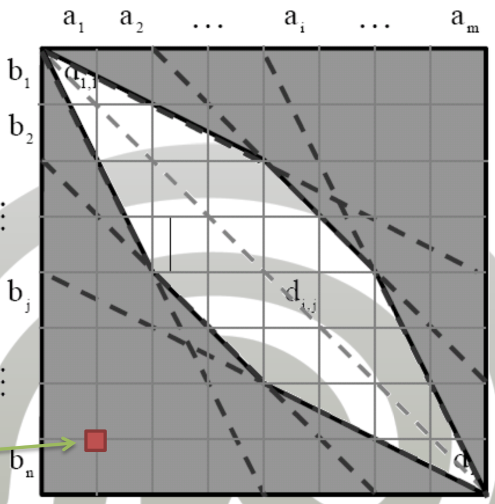
Optimization 1:
- Apply operations from left to right string
- \( O(mn) \) vertices in graph
- Costs are non-negative
- Use Dynamic programming:
  - Mongeau/Sankoff, 1990
  - Consider all possible nodes in graph regardless of costs
  - Ignore nodes with very high cost
  - Costs near the diagonal are candidates for the minimum
Optimization 2:
- Adapt costs to typical errors
  - R...R -> R typical error (consolidation)
- UD/DU is no typical error -> higher cost
- Inserting R cheaper than inserting U/D
- Replacement of R->D and R->U cheaper than U->D/D->U (U/D should be treated the same)
- Similar costs for fragmentation/consolidation
- Similar costs insertion/deletion

../_images/08-parsons.png

Improvement: Difference Codes¶

Problem with Parsons code:
- Ignore strength of pitch change
Idea:
- Store interval information as number of semitones (12-tone scale)
- e.g., \( \Diamond,0,1,2,0,-2,-1,-2,-2 \)
Kosugi et al., 2000
- Research of distribution of intervals in music
- Database with 10000 songs
- Result: Gaussian distribution
  - \( \pm 2 \) semitones (1 whole tone) very often
  - Tritones (\( \pm 6 \) semitones) very rare (very un-harmonic)
Advantage
- Precise distinction
  - Using weighted edit distance
  - Weight: Size of the jump
Disadvantage
- More expensive
- Depends on the audio collection (may not matter/humming may be too coarse)

Frame-based Representation¶

Idea:
- Use contour of music
- e.g., pitch curve
- Match two series of different length
Representations:
- Use time series of pitch values (frames)
- Frame should be equidistant (e.g., 50 ms)
Advantage:
- No incorrect segmentation
- Rhythm information can be contained
Disadvantage:
- Higher retrieval time
Problem of point-wise comparison:
- Different speed of query
- Different rhythm in query
Solution: Dynamic matching
- Dynamic Time Warping

Dynamic Time Warping¶

Berndt/Clifford, 1994
- Distance measure for time series
- Same principle like edit edit (but no finite alphabet for operations)
- Operation cost: Depend on values
- Match pairs of points / assign each point in the one signal a point of the other signal

Formal¶

Time series
- \( f(t) \) with \( N \) points: \( f_1,\ldots,f_N \)
- \( g(t) \) with \( M \) points: \( g_1,\ldots,g_M \)
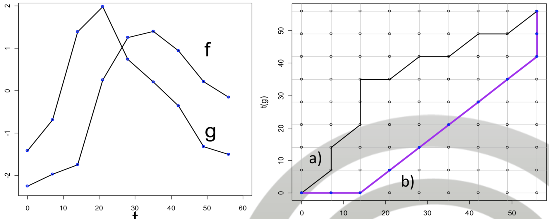
Warping diagram:
- Grid \( N\times M \)
- Axis:
  - \( t_f =1,\ldots,N \)
  - \( t_g=1,\ldots,M \)
- Each point \( (i,j) \) maps \( f_i \) to \( g_j \) (\( f(i) \) to \( g(j) \))
Warping path \( W \):
- Series of points \( (i,j)\subsetneq \mathbb{N}_N\times\mathbb{N}_M \)
- \( K \) number of points
- \( W=((i_1,j_1),\ldots,(i_K,j_K)) \)
Warping properties (of the warping path):
- \( 1\leq k \leq K \)
- Monotony
  - Only move forward
  - \( i_k \leq i_{k+1} \) (analog to \( j \))
- Continuity
  - Do not leave points out
  - \( i_{k+1}-i_k\leq 1 \) (analog to \( j \))
- Boundaries
  - Match start and end
  - \( i_1=j_1=1 \) (map \( f(1) \) to \( g(1) \))
  - \( i_K=N \) (map \( f(N) \) to \( g(M) \))
  - \( j_K=M \)
Calculation
- Dynamic programming \( O(nm) \)

../_images/08-warping.png

Uniform Time Warping¶

Idea:
- Warping path as diagonal as possible
- Prefer consecutively matching of points (cf. edit distance)
- Uniformly match the series: Stretch series uniformly to \( mn \) points
Generalization of time scaling
Time series \( x_n \) and \( y_m \)
Distance: \( d^2_{UTW}(x,y)=\frac{1}{mn} \sum_{i=1}^{mn} (x_{\lceil i/m \rceil}-y_{\lceil i/m \rceil})^2 \)
Difference between every two points
- Each point \( x_i \) is replicated \( m \) times
- Each point \( y_i \) is replicated \( n \) times
Problem: Variable speed of the time series ==Why???==

Local-dynamic Time Warping¶

Idea:
- Extend series to same length (as in UTW)
- Compare point-wise with little warping intervals
- Prefer diagonal matrix
Complexity \( O(kn) \)
- \( k \): Width of band around diagonal (called slope constraint)
- Slope constraint: Match a point to at most \( k \) other points
Zhu/Shasha, 2003
- GEMINI approach
- Map the query into an envelope
- ==What was the contribution?==

Hidden Markov Models¶

Motivation:
- Frame-based representations shows the behavior of audio signal but no interpretation
- e.g., we do not know whether a certain pitch is the start of a note, its hold or its decrease
- What caused a certain pitch?
  - e.g., Attack phase, an independent note or noise?
Idea:
- Idea: See melody as stochastic process
- Purpose of HMMs: Match a real-world observation to a stochastic process
Goal:
- Model acoustic events (semantic events in the music; notes)
- Detect the melody of a sequence of pitches
Scenario/representation:
- Simplicity: Focus on hull curve for a single tone/note (ADSR)
- Assume a hidden sequence of real acoustic events (string, fixed alphabet) generating the observations
- Alphabet of envelope: \( Q=\{A, D, S, R, \epsilon\} \) (\( \epsilon \) is silence)
- Acoustic event single note represented by sequence of atomic events over \( Q \)
- Use Markov chain for state transitions
Problem:
- Detection of acoustic events from signal is not possible
- Solution:
  - True Markov model is unknown (hidden)
  - State selection must be probabilistic (derive hidden state sequence from signal)
  - e.g., Observe pitch \( x \), in which state of the HMM are we?
Three Problems
- Likelihood (select model)
- Decoding (select state sequence)
- Learning (select parameters)

../_images/08-adsr.png

Problem Statement¶

Terminology:
- Observation: Recognized pitch/amplitude (\( o_i \) is pitch at time step \( i \))
- State: State/phase of the note creation from the hull curve
Problem statement:
- Given sequence of observations \( (o_{i_1},\ldots,o_{i_n})\in O^n \)
- Find sequence \( (q_{j_1},...,q_{j_n})\in Q^n \) with maximal probability for generating the sequence of observations
Example:
- Observation \( o_3 o_5 o_1 \)
- Possible state sequence \( ADS \)
- \( P=\pi(A)\cdot p_A(o_3) \cdot P_{A,D} \cdot p_D(o_5) \cdot P_{D,S} \cdot p_S(o_1) \)

Formalization¶

Conditional probability:
- \( P(A|B)=\frac{P(A\cap B)}{P(B)} \)
Stochastic process:
- Sequence of random variables \( (X_0,X_1,X_2,\ldots) \)
Markov process:
- Stochastic process satisfying the Markov condition
- Independence of previous steps/states
Markov condition/property:
- \( \forall n\in \mathbb{N}_0, i_0,...,i_{n+1}\in I \) with \( P(X_0=i_0,...,X_n=i_n) > 0 \): \( P(X_{n+1}=i_{n+1}|X_0=i_0,...,X_n=i_n) = P(X_{n+1}=i_{n+1}|X_n=i_n) \)
- Probability for transition into next state depends only on present state
‌Homogeneous Markov process:
- Transition is independent of \( n \) (e.g., time-invariant)
- Initial distribution \( \pi=(\pi)_{q\in Q} \)
- \( P(X_0=i_0,\ldots,X_n=i_n) = \pi_{i_0}\cdot p_{i_0 i_1}\dots p_{i_{n-1}i_n} \)
Hidden Markov Model components:
- Homogeneous Markov process:
  - \( (Q_t)_{t\in\mathbb{N}} \)
  - State set \( \mathcal{Q}=\{q_1,...,q_N\} \)
  - \( N \) states
  - \( Q_i:\Omega\rightarrow\mathcal{Q} \)
  - Note: Random variable \( Q_i \) represents distribution depending on the time (at time step \( i \))
- Transition probabilities:
  - \( a_{ji} = P(Q_t=q_i|Q_{t-1}=q_j) \)
  - \( \sum_{i=1}^N a_{ji} = 1 \)
- Start distribution:
  - \( \pi_i=P(Q_0=q_j) \)
  - e.g., in audio probability for attack is \( Q(A)=1 \)
- Stochastic process of observations:
  - \( (O_t)_{t\in\mathbb{N}} \) of observations
  - Set of observations \( \mathcal{O}=\{o_1,...,o_M\} \)
  - \( M \) observations
  - \( O_i:\Omega\rightarrow \mathcal{O} \)
- Observation probabilities:
  - Observation probability of observation \( o_k \) in state \( q_j \)
  - \( b_j(k)=P(O_t=o_k\mid Q_t=q_j) \)

Likelihood¶

Problem:
- Given: Observation sequence and a HMM
- What is the probability that the HMM generated observation sequence?
- \( P(O\mid\lambda) \)
Use case:
- Select between different models
Idea:
- Walk over all possible state sequences
Formal:
- \( T \) time steps
- Observation sequence \( o=o_{i_1},\ldots,o_{i_T}\in \mathcal{O}^T \)
- HMM \( \lambda \)
Proof:
- Assume state sequence \( q_{j_1},\ldots,q_{j_T}\in \mathcal{Q}^T \)
- \( P(O_1,\ldots,O_T|Q_1=q_{j_1},\ldots,Q_T=q_{j_T}) \)
- \( =\Pi_{k=1} P(O_k|Q_1=q_{i_1},\ldots,Q_T=q_{j_T}) \) (Markov property, independent transitions)
- \( =\Pi_{k=1}^T P(O_k|Q_k=q_{j_k}) \)
- \( =\Pi_{k=1}^T b_{j_k}(i_k) \)
Result:
- \( P(O_1=o_{i_1},\ldots,O_T=o_{i_T}) \)
- \( =\sum_{q_{j_1},\ldots,q_{j_T}} \pi_{j_1}\cdot b_{j_1}(i_1)\cdot a_{j_1,j_2}\cdots b_{j_T}(i_T) \)
- Compute using the Forward algorithm in \( O(N^2T) \)

Decoding¶

Most probable state sequence
Problem:
- Observation sequence \( o=o_{i_1},\ldots,o_{i_T}\in \mathcal{O}^T \)
- HMM \( \lambda \)
- What is the state sequence \( q \) that generates the observation sequence \( o \) with highest probability?
- Tilo: What is the best explanation for the observations?
Use maximum likelihood estimator:
- \( P_\lambda(Q_1=q_{j_1},\ldots,Q_T=q_{j_T}\mid O_1=o_{i_1},\ldots,O_T=o_{i_T}) \)
- Maximize this term
Formalization:
- \( P(Q,O)=P(Q|O)P(O)=P(O|Q)P(Q) \)
  - \( P(O) \) is constant (observation sequence given)
  - Maximize \( P(Q,O) \) instead of \( P(Q|O) \)
- \( \delta_t(j)=\max_{q_{j_1},\ldots,q_{j_{t-1}}} P(Q_1=q_{j_1},\ldots,Q_{t-1}=q_{j_{t-1}}, Q_t=q_j, O_1=o_{i_1},\ldots,O_t=o_{i_t}) \)
- \( \delta_{t+1}(j)=(\max_{1\leq i\leq N} \delta_t(i)a_{ij})\cdot b_j(i_{t+1}) \)
  - Maximum probability \( \cdot \) transition \( \cdot \) observation
- \( \delta_t(i) \): Probability of the most probable path to state \( q_i \) in time \( t \)
- \( \max_{1\leq i\leq N} \delta_T(i) \) Probability of the maximal probable state sequence
- Use dynamic programming for \( \delta_t(i) \)
Use Viterbi algorithm

Viterbi algorithm¶

Viterbi, 1967
Idea:
- Maximum likelihood estimator + dynamic programming
\( \delta_t\in[0,1]^N \): Vector containing the maximal probability of observing \( o_i \) at time \( t \) in state \( q_i \)
\( \psi_t\in[0,1]^N \): Most probable state at time \( t-1 \) (previous state)
Steps:
1. Initial Step
  - For all \( 1\leq j\leq N \)
  - \( \delta_1(j)=\pi_j b_j(i_1) \)
  - \( \psi_1(j)=0 \)
2. Induction
  - For all \( 2\leq t\leq T,1\leq j\leq N \)
  - \( \delta_t(j)=(\max_{1\leq i\leq N} \delta_{t-1}(i)a_{ij})\cdot b_j(i_t) \)
  - \( \psi_t(j)=\arg\max_{1\leq i\leq N} \delta_{t-1}(i)a_{ij} \)
3. Termination
  - \( p=\max_i \delta_T(i) \)
  - \( j_T=\arg\max_i \delta_T(i) \)
4. Path definition (recursive)
  - Final path \( q_{j_1},\ldots,q_{j_T} \)
  - \( \forall 1\leq t\leq T-1: j_t=\psi_{t+1}(j_{t+1}) \)

Learning¶

Goal:
- Determine transition-, observation- and start probabilities
Given: Training sequence \( o=o_{i_1},\ldots,o_{i_T}\in \mathcal{O}^T \)
Task:
- Determine model parameters \( \lambda=(A, B, \pi) \) maximizing \( P(o)=P_\lambda(O_1=o_{i_1},\ldots,O_T=o_{i_T}) \)
- High-dimensional optimization problem
- \( A \): Matrix for transition probabilities
- \( B \): Matrix for observation probabilities
- \( \pi \): Vector of starting probabilities
Use Baum-Welch algorithm

Baum-Welch algorithm¶

Baum et al., 1970
Compute local optimum
Terminology:
- Forward variable:
  - Probability of observing the first part of the training sequence resulting in current state
  - Move from start to latest state
  - How did I got the state \( t \)?
- Backward variable:
  - Probability of observing the rest of the training sequence from current state
- Both represent the whole path
Formalization:
- Forward variable:
  - \( \alpha_1(j)=\pi_j\cdot b_j(o_{i_1}) \)
  - \( 1\leq j\leq N:\alpha_t(j)=P(O_1=o_{i_1},\ldots,O_t=o_{i_t},Q_t=q_j) \)
  - \( 1\leq t \leq T-1,1\leq j\leq N: \alpha_{t+1}(j)=(\sum_{i=1}^N\alpha_t(i)a_{ij})\cdot b_j(i_{t+1}) \)
  - for \( 1\leq t\leq T-1 \) and \( 1\leq j\leq N \)
- Backward variable:
  - \( \beta_t(j)=P(O_{t+1}=o_{i_{t+1}},\ldots,O_T=o_{i_T}|Q_t=q_j) \)
  - \( 1\leq j\leq N:\beta_T(j)=1 \)
  - \( \beta_t(j)=\sum_{i=1}^N a_{ji}b_i(i_{t+1})\beta_{t+1}(i) \)
  - for \( 1\leq t\leq T-1 \) and \( 1\leq i\leq N \)
- \( \gamma_t(j) \)
  - Probability of being in state j at time t
  - Multiplication of \( \alpha \) and \( \beta \)
  - \( =P(Q_t=q_j|O) \)
  - \( =\frac{P(o, Q_t=q_i)}{P(O)} \)
  - \( =\frac{\alpha_t(j)\beta_t(j)}{P(O)} \)
  - \( =\frac{\alpha_t(j)\beta_t(j)}{\sum_{k=1}^N \alpha_t(k)\beta_t(k)} \)
- \( \xi_t(i,j) \)
  - Probability to be at time \( t \) in state \( q_i \) and in time \( t+1 \) in state \( q_j \)
  - Note: to \( q_i \) by \( \alpha \), from \( q_j \) to end by \( \beta \)
  - Denominator: Move \( t \) over the observation sequence, all possibilities to transition between the states
  - \( =P(Q_t=q_i,Q_{t+1}=q_j|o) \)
  - \( =\frac{\alpha_t(i)a_{ij}b_j(i_{t+1})\beta_{t+1}(j)}{P(o)} \)
  - \( =\frac{\alpha_t(i)a_{ij}b_j(i_{t+1})\beta_{t+1}(j)}{\sum_{k=1}^N \sum_{l=1}^N \alpha_t(k)a_{kl}b_l(i_{t+1})\beta_{t+1}(l)} \)
- Expected value of outgoing transitions of \( q_i \):
  - \( \sum_{t=1}^{T-1}\gamma_t(i) \)
- Expected value of transitions from \( q_i \) to \( q_j \):
  - \( \sum_{t=1}^{T-1}\xi_t(i,j) \)
Steps:
1. Initial state estimate
  - Random or additional knowledge
  - \( \pi_i^0, a_{ij}^0, b_j^0(k) \)
  - \( 0 \): Training step
2. Re-estimate parameters
  - Iterate over \( r\geq 0 \)
  - \( \gamma_t^r(i) = \frac{\alpha_t^r(i)\beta_t^r(i)}{\sum_{k=1}^N \alpha_t^r(k)\beta_t^r(k)} \)
  - \( \xi_t^r(i,j)=\frac{\alpha_t^r(i)a^r_{ij}b_j^r(i_{t+1})\beta_{t+1}^r(i)}{\sum_{k=1}^N\sum_{\ell=1}^N \alpha_t^r(k)a_{k\ell}^r b^r_\ell(i_{t+1})\beta_{t+1}^r(k)} \)
  - \( 1\leq i\leq N: \pi_i^{r+1}=\gamma_1^r(i) \)
  - \( 1\leq i\leq N: a_{ij}^{r+1}=\frac{\sum^{T-1}_{t=1} \xi_t^r(i,j)}{\sum_{t=1}^{T-1} \gamma_t(i)} \)
  - \( 1\leq i\leq N: b_i^{r+1}(k)=\frac{\sum^{T-1}_{t=1} (\gamma_t(i)\cdot \hat{P}(O_t=o_k))}{\sum_{t=1}^{T-1} \gamma_t(i)} \)
    - \( \hat{P}(O_t=o_k) = 1 \) if \( o_k \) was observed, otherwise \( \hat{P}=0 \)
3. Termination
  - For each step, we have HMM \( \lambda^r \)
  - \( P_{\lambda^{r+1}}(o)\geq P_{\lambda^r}(o) \)
  - Each iteration, the model gets better
  - Iterate until parameters change too little

Application¶

HMMs Types¶

‌Ergodic model
- Complete HMM (fully meshed)
‌Bakis model
- Left-right HMM
- \( \forall j<i:a_{ij}=0 \)
- Good for time-varying signals (e.g., music, speech)

Workflow¶

Pitch is the observation (e.g., 700 Hz)
Note is the acoustic event (e.g., note D)
Feature extraction:
- Convert raw signal to sequence of observations (string)
- Describe the implementation of an acoustic event by a state sequence of a HMM
- e.g., 36 states for three octaves (state = tones)
Acoustic events:
- Determine acoustic events in the observations (automatic vs. manual)
- Mapping between parts of the observation and an acoustic event (generate the training set)
Training
- Train \( H \) different HMMs \( \lambda_1,\ldots,\lambda_H \)
- One HMM per acoustic event (e.g., note)
- Automatic detection of events: Large \( H \)
- Manual detection of events: Small \( H \)
- Use Baum-Welch algorithm
Matching:
- Compute the Likelihood of each HMM \( \lambda_i \)
- Use the acoustic event with the highest likelihood HMM

Macro-HMM¶

Combination of multiple HMMs
- Behaves like a normal HMM
- each state in macro HMM is a HMM (e.g., tones)
- Combine with equal probabilities
Use the macro-HMM to detect the melody of a sequence of pitches
Feature extraction (detect melody):
- \( H \) different HMMs
- Observation sequence: \( o_{i_1},\ldots,o_{i_T}\in \mathcal{O}^T \)
- Find sequence \( ((l_1,t_1),\ldots,(l_R,l_R))\in(\mathbb{N}_H\times \mathbb{N}_T)^R \)
- \( (l_i, t_i) \) associates HMM \( \lambda_{l_i} \) with the observations \( o_{t_i} \) to \( o_{t_{i+1}} \)

Problems¶

Infinite sequence of observations
- Not clear, where events start
- e.g., window over a data stream, Shazam
- Idea:
  - Build sub-sequences using sliding windows
  - Viterbi for each sequence
- High complexity (look at all subsequences)
  - \( O(w\cdot|\sum^H_{i=1} |\lambda_i||) \)
Window size for sub-sequences
- Must be sufficiently large
- Traverse HMMs until a sufficiently large probability occurs (then return that HMM)
- Try to walk through different states