Image Retrieval
Basics
- Image representation: Matrix with color values
- Low-level features:
- Idea: How are images described with natural language?
- Color (foreground, background)
- Shapes
- Texture (contrast, repetition)
- Problem:
- Loss of information/semantics
- Low-level feature combination works better
- Use LLF to exclude images
- Idea: How are images described with natural language?
- High-level features:
- Wavelets
- Fourier transformation
- Input: Image (as signal)
- Position space to frequency domain
- Similarity search / matching
- Exact matching is easy
- Similarity not
Color-based Retrieval
Basics
- Assumption: If two images share the same color, their content is similar
- Problem: Loss of information (e.g., sunset vs sunrise)
- Color:
- Event with three participants
- Light (property)
- Object (property)
- Observer
- Important for human perception
- Event with three participants
Color Spaces
- Motivation:
- Required to work with colors (e.g., add lightning)
- Describe and compare colors mathematically
- Definition: Multi-dimensional space to describe color components
- Requirement for MMDBs: Distance in a color space should correlate to distance in perception
- Perception: Three receptors for wavelengths
- Blue (435 nm)
- Green (546 nm)
- Red (700 nm)
RGB
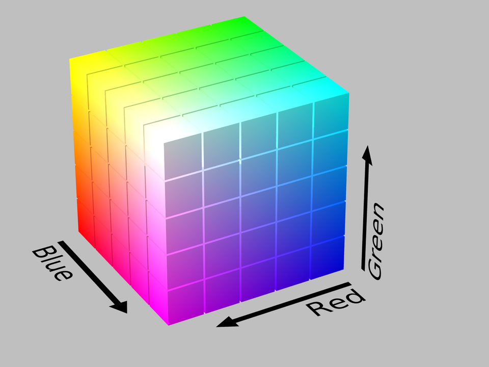
- Euclidean vector space
- Additive color mixing
- Red, Green, Blue (\( 0-255 \))
- Advantage
- Good representation of visible light
- Disadvantage
- Poor for similarity search (equal distance is no equal similarity change, magenta vs. blue/red)
CMYK
- Cyan, Magenta, Yellow, Black/key
- Subtractive color model
- Represent painting ink
Munsell Color System
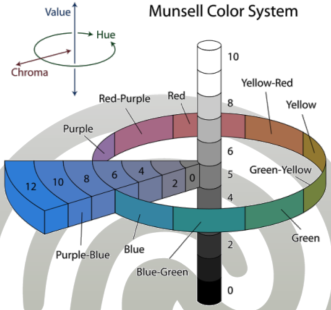
- Munsell, 1905
- Idea:
- Create color space respecting human perception (transform RGB)
- Distance in color space is distance in perception
- Problem: No known color space with uniform perception
- Creation: Humans sort colors
- Dimensions:
- Chroma (i.e., saturation)
- Hue
- Value (black to white)
- Use cases
- Hair color / skin color
- Color of liquids
- Disadvantages
- Distances between non-adjacent colors don’t respect perception
- No simple transformation to RGB
CIE Color space
- Commission Internationale de l’eclairage (Standardization Commission on Illumination)
- Idea:
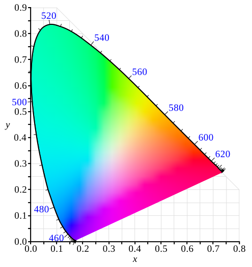
- Propose perceptional space
- Based on opponency + thrichromacy
- CIE 1976 (L*, a*, b*)
- L: Lightness (0-100)
- a*: green (negative value) to magenta (positive value)
- b* blue (negative value) to yellow (positive value)
- Successful color model (implemented in Photoshop)
- Non-linear transformation from RGB
HSV Color space
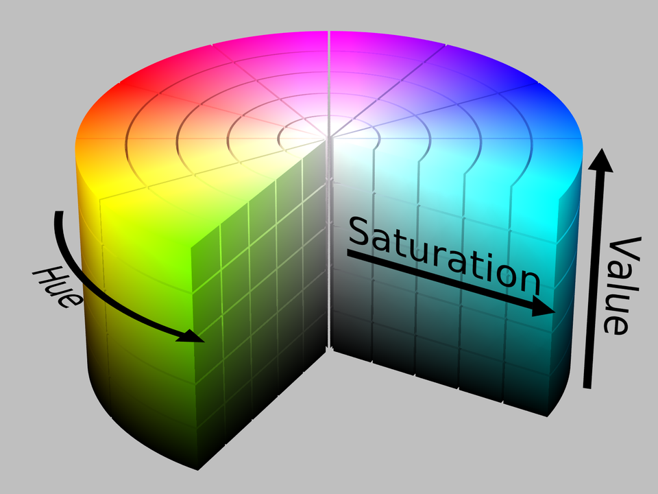
- Simpler than CIE
- Hue, saturation, value
- Non-linear transformation from RGB (but easy to compute)
- Advantage
- Intuitive/easy
- Nearly perceptional
- Good for similarity search
- Used in MPEG-7 (color space for image descriptors)
Color Features
- Problem:
- Image has many pixels
- Pixel-by-pixel-comparison is too expensive
- Solution: Aggregate color
- Color channel metric (e.g., average)
- Color histogram
- Color layout/regions
- Important trade-off:
- Complexity of calculation (e.g., average color, quadratic distance)
- Accuracy of description (e.g., cross-talk matrix has more semantics)
Color Channel Metrics
- Idea: Represent image by vector of three components
- Moments:
- Mean-color-distance (average color)
- Variance-color-distance: \( \sigma_R^2, \sigma_G^2, \sigma_B^2 \)
- Skewness-color-distance
- Comparison: Euclidean distance
- Experiment Castelli/Bergmann:
- Color channel metrics have bad retrieval accuracy
- Minkowski/Quadratic distance are similar
Average Color
- Compute average color of all pixels
- \( C_{avg} = (R_{avg}, G_{avg}, B_{avg}) \)
- Advantage: Simple
- Disadvantage: Very bad measure (perceptionally insufficient)
- Use case:
- Exclude/prune images using average color (dominant color influences average color)
Color Histogram
- Use histogram of colors
- Represents number of pixels with certain color
- Represents a global description of the image
- Normalization
- Used for comparison
- Normalize by number of pixels
- Sum of columns equals one
- RGB:
- 16 million colors too much
- Reduce number of columns, i.e., color quantization
- Problem: Transform vector to column
- Solution: Color quantization
- Comparison using metrics (distance functions):
- Minkowski distance
- Quadratic distance
- Mahalanobis distance
Color Quantization
- Purpose:
- Reduce number of columns in histogram
- Merge similar colors (e.g., quantize vector space)
- Mapping from k-dim. space to color partition
- Formal
- Code words/Codebook (columns) \( C=\{y_0,...,y_{m-1}\} \)
- Encoding/Code \( Q_C \)
- \( Q_C^m: \mathbb{R}^k \rightarrow C \)
- Requirements
- Group perceptionally similar colors together
- Codeword should be best representation of color
- Minimize number of partitions (increase search efficiency)
- Quantization HSV
- \( Q_C^{166} \) (Smith, 1997)
- Hue: 18 segments (each 20°)
- Saturation: 3 segments
- Value: 3 segments
- Gray: 4 segments
- Saturation is zero
- Hue can be any value for gray
- Group perceptionally similar
- \( 0\leq 25 \leq 50 \leq 75 \leq 100 \)
- Quantization RGB (idea)
- Use k-means centroids as code words
- Enumerate clusters
- Use k-NN on other images to sort into code words
Minkowski distance
- Histogram \( h_1, h_2 \)
- Histogram as vector
- Usually, \( r\in\{1,2\} \)
- Personal Idea: Consider weighted Minkowski distance
- Weight different colors
- e.g., collection of leafs (focus on greenish colors, ignore red/yellow/blue noise)
- Counterargument: red/yellow/blue may be important for discrimination/differentiation
- Disadvantage:
- Does not respect color similarity (e.g., distance between red and bright red is equal to red and blue)
- Works poorly for color shifts (i.e., higher/lower saturation)
- Advantage
- Sufficient for MMDBMS
Quadratic measure
- Idea: Use similarity of different colors
- Use cross-talk matrix \( A \)
- Pairwise similarity \( a_{i,j} \) between colors \( y_i \) and \( y_j \)
- \( a_{i,i}=1 \)
- \( a_{i,j}=a_{j,i} \)
- Formula
- \( d_A(h_1, h_2) = (h_1-h_2)^T \cdot A \cdot (h_1-h_2) \)
Mahalanobis distance
- Observation: Color combinations with high covariance don’t contribute to discrimination
- Idea:
- Co-occurring colors should receive low weight
- Use covariance matrix \( \Sigma^{-1} \) as cross-talk matrix
- Generate covariance matrix using a representative set of images (histograms) from the collection
- Formula
- \( d_M(h_1, h_2) = (h_1-h_2)^T \cdot \Sigma^{-1} \cdot (h_1-h_2) \)
- Covariance matrix:
- All colors un-correlated:
- Diagonal matrix
- Norm is quadratic weighted Euclidean distance (weighted by standard deviation of the respective color)
- Some colors correlated:
- Transform coordinate system
- Reduce correlating colors to one dimension (e.g., PCA / SVD)
- Result: New basis vectors are uncorrelated
- In reduced space, the distance is weighted by the eigenvectors \( \lambda \)
- Weighted Euclidean distance in reduced space is Mahalanobis distance in original space
- All colors un-correlated:
Color regions
- Idea:
- Divide image into regions (individual description)
- Object of interest is in focus/the middle of the image
- Take semantics of an image into account
- Calculation: Use weighted sum of similarity of regions
- Different regions can be weighted
- e.g., foreground is more important
- Approaches
- Grid distribution (Hsu et al., 1995)
- Divide image into grid
- Weight regions differently
- Common compositions (Stricker/Dimai, 1996)
- e.g., foreground motif
- Fuzzy regions (image)
- Weighted regions
- Grid distribution (Hsu et al., 1995)
Texture-based Retrieval
Texture
- Definition
- Recurrent, typical, obvious (clearly visible) pattern in picture
- Often used to describe images
- Research
- Texture segmentation
- Find areas with homogeneous textures
- Decomposition of image
- Color and texture are related (can be combined for features)
- Texture classification
- Denote homogeneous textures with text or
- Describe homogeneous textures with features
- e.g., Ice, water, tomography
- Semantic classification
- Represent objects from the real world (e.g., corn, water)
- Application-dependent
- Descriptive classification
- No direct meaning (e.g., parallel)
- Can be used for query-by-example
- Ensure comparability between image collections
- Texture synthesis (create textures)
- Texture segmentation
- Criteria for a texture (Rao/Lohse, 1993)
- Repetition
- Orientation (e.g., vertical)
- Complexity (e.g., how regular?)
- Features
- Low-level
- Julesz’ Texton
- Tamura-measure
- Random field model
- High-level
- Gabor-filter
- Fourier transform
- Wavelet transform
- Low-level
Low-level features
Julesz’ Texton
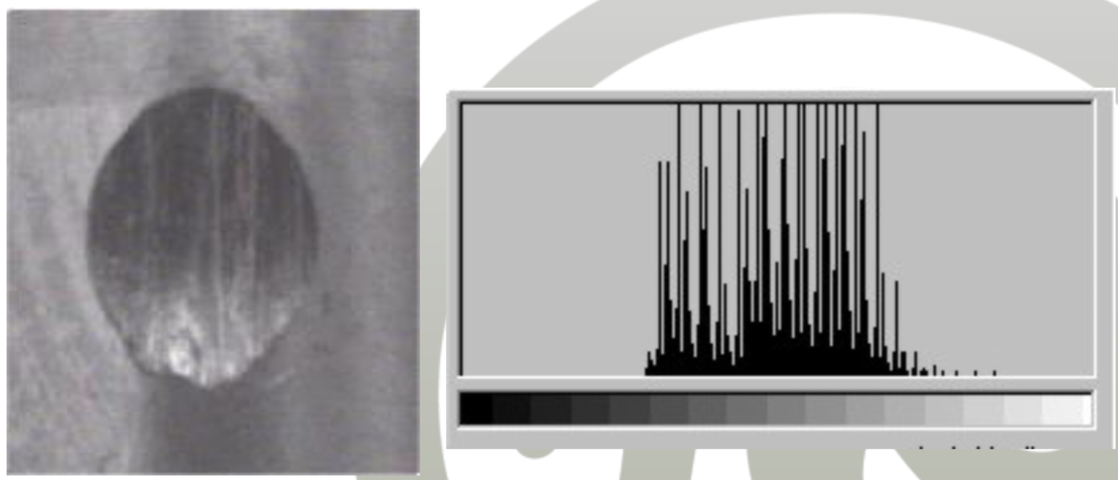
- Also called grey-level analysis
- Grey-level: Intensity of pixel
- Idea:
- Create grey-level histogram (distribution)
- Use moments of distribution for description
- Histogram of grey values
- Claim: Similar pattern produce similar distribution of grey values
- Problem: Distribution ignores position
- Problem: Repetition can’t be seen
- Grey-level co-occurrence matrix \( C_d \)
- Matrix for a specific distance \( d \)
- Cell \( a_{ij} \) indicating how often grey-level \( i \) co-occurs with grey-level \( j \) for points with Euclidean distance \( d \)
- Consider all pairs of points with Euclidean distance \( d \)
- Julesz, 1961:
- Empirical probability distribution of intensity change to the right
- Use position
- \( P(I(s) = i \land I(s+d)=j) \)
- Julesz, 1975:
- Generalization to any directions
- Julesz, 1973
- Thesis: Texture with identical grey-level co-occurrence matrices => People can’t distinguish
- Thesis is wrong (Julesz, 1981)
- Can be used as rule of thumb
- Problem: Texture is more complex than just the intensity distribution
Tamura Measure
- Tamura et al., 1978
- Describe texture with dimensions:
- Granularity (e.g., gravel vs. sand)
- Contrast (sharpness)
- Directionality
- Line-Likeness (ignore)
- Regularity (ignore)
- Roughness (ignore)
- Matching
- Granularity, Contrast and directionality are un-correlated
- Image
- \( d_\text{texture}^2(x,y) = \frac{(G_x-G_y)^2}{\sigma_G^2}+\frac{(C_x-C_y)^2}{\sigma_C^2}+\frac{(D_x-D_y)^2}{\sigma_D^2} \)
- Divide by standard deviation to normalize the components, e.g., granularity is a window size and directionality is a ratio between zero and one
Granularity
- Example: Areal photo from different heights
- Granularity:
- Also called coarseness
- Size of the objects in the texture
- Idea:
- Neighborhood influences the granularity
- Observe neighborhood for brightness changes
- Try to find the size of the objects in the texture (e.g., checkerboard: size of one square)
- Calculation
- Idea: Look at the brightness of left/right pixel, to see if they change, if there are different objects
- Use windows of sizes \( 2^i \times 2^i \)
- For each pixel and every window size \( 0\leq i\leq 5 \), compute the average gray value
- For each pixel, compute difference of grey-level means of all adjacent windows
- Vertical: \( y+2^{i-1}, y-2^{i-1} \)
- Horizontal: \( x+2^{i-1}, x-2^{i-1} \)
- \( \delta_i^h, \delta_i^v \)
- Compute the window size maximizing the difference of means in either direction
- \( S_{best} = 2^i \) with \( i=\arg_i\max \{\delta_i^h,\delta_i^v\} \)
- Granularity of entire image:
- Mean of maximum window sizes of al pixels
- Histogram of pixels and their maximum window size
- Each pixel is assigned exactly one maximum window size
- Finer-grained comparison
- Meaning of the window size:
- Size of the objects in the texture (e.g., circles, squares, etc.)
- Window size larger than the granularity: Similar distribution of grey levels
- Window size smaller than granularity: No difference or very high difference
- Problem: Small images lead to small granularity
- Reason: The window size can’t be large
- Equitz/Niblack, 1994
- Estimation of \( \delta_i \) for smaller images
Contrast
- Visual:
- Clarity of image
- Sharpness of color transitions
- Exposure
- Shadows
- Grey-level distribution:
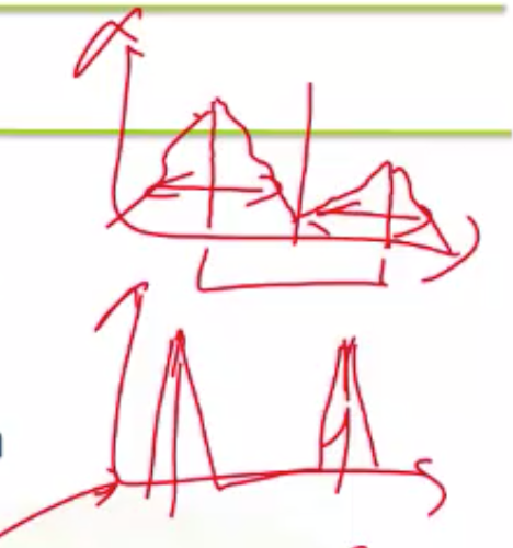
- Low contrast: Flat peaks
- High contrast: Sharp peaks
- Use higher-order moments of grey-level distribution
- Contrast: \( K=\frac{\sigma}{\sqrt[4]{\alpha_4}} \)
- \( \sigma \): Standard deviation on collection
- \( \alpha_4 = \frac{\mu_4}{\sigma^4} \): Kurtosis
- \( \mu_4 \): Fourth central moment
- Can differentiate Uni- and Bi-modal distributions
Directionality
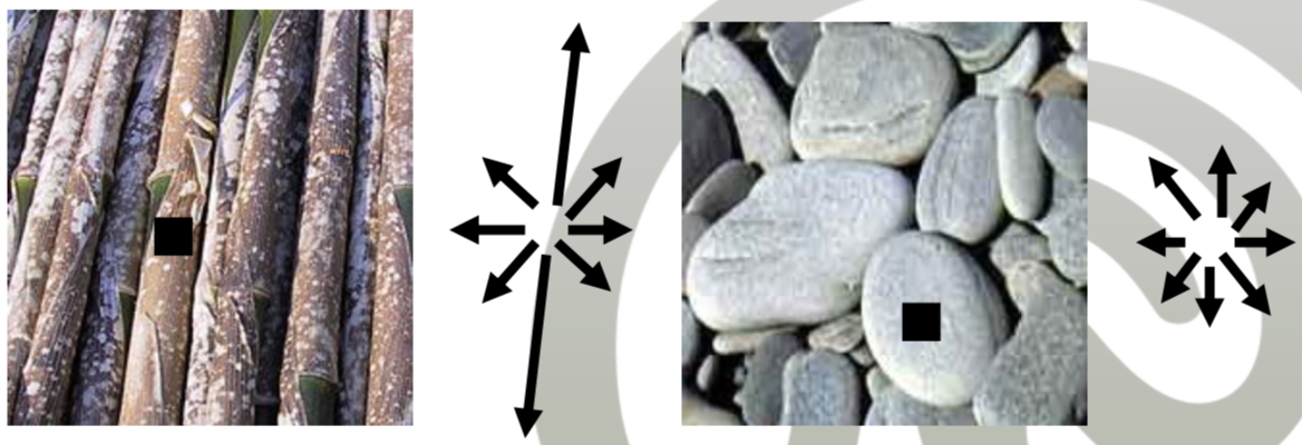
- Find predominant direction of elements
- Example:
- Trunks: Highly directional
- Stones: Weak directional
- Description for the gradient of each pixel
- Angle (direction)
- Magnitude (strength)
- Computation
- Idea: How many pixels can I go in a certain direction without exceeding a certain gradient?
- Compute gradient of color for a set of angles
- Histogram with number of pixels exceeding a threshold per angle (Morris: number of pixels below a certain threshold)
- Dominant direction: Peak in histogram
- Problem: Rotated images
- Rotated image has different dominant direction
- Results in bad retrieval results
- Use number of peaks and peak amplitude (bar height) for images
Random-Field model
- Stochastic/probabilistic model
- Use repeating/recurrent nature of texture
- Idea:
- Use generative model for texture synthesis
- Assume, a model generated textures in collection
- Use model parameters for description/matching
- Comparable to IR language models
- Generative model
- Good model: Create different but similar textures
- Predict pixel color/intensity by neighborhood
- Random field
- \( F \) is matrix with pixel intensities from image
- \( F \) is random variable
- Called random field
- Known distribution
- Unknown parameters
- Maximum likelihood estimation:
- Given an image
- Find the parameters for \( F \) that generated the image best
- Markov property
- Event does not depend on complete history of events
- Only depends on the last k events
- e.g., sufficiently regular textures require only the neighborhood/locality pixels
- Neighborhood shifts \( N\subset \mathbb{Z} \times \mathbb{Z} \)
- Neighborhood \( N_s = \{s+t\mid t\in N\} \)
- Assumptions:
- Markov condition is valid
- Size of neighborhood is well chosen
- Models:
- Simultaneous AutoRegressive model (SAR)
Simultaneous AutoRegressive Model (SAR)
- Popular class of models for texture description
- auto-regression: self-similar
- Idea:
- Function depends on its own
- Formal
- \( F(s) \): Value of pixel \( s \)
- \( W(s) \): Random variable for noise (mean 0, variance 1)
- \( \theta(t), \beta \): Parameters
- \( F(s) = \sum_{t\in N} \theta(t) \cdot F(s+t)+\sqrt{\beta}\cdot W(s) \)
- Computation:
- Minimization problem
- Idea: Compute using the least squares method
- Problem: Neighborhood size different to estimate
- Neighborhood size must reflect texture size
- Small texture vs. large texture
- Solution: Mao/Jain, 1992 (Multi-resolution simultaneous autoregressive model)
- Advantage:
- Good low-level description of textures
High-level features
Basics
- Goal: Describe complete picture without information loss
- Image as input signal
- \( f:\mathbb{N}\times \mathbb{N} \rightarrow [0,1] \)
- Image row is sequence of real numbers (intensity)
- Image is discrete function
- Color space: One function per component
- Polynomial interpolation
- Transform sequence of numbers into polynomial
- Problem: Polynomial not suitable for shape representation
- Textures are recurrent/periodic
- Polynomials are not periodic
- Other transformations
- Discrete Fourier Transform
- Discrete Cosine Transform
- Wavelet Transform
Discrete Fourier Transform
- Fourier transform can be generalized to two-dimensional data
- Each pixel has direction and wavelength of oscillation
- Results in \( A(i,j), B(i,j) \) indicating amplitude of sine/cosine wave
- Compare using an image
- Instead of matrices \( A \) and \( B \)
- Pixel value \( (i,j) \) is length of vector \( (A(i,j), B(i,j)) \)
- Properties of frequency space:
- Centered on fundamental frequency
- Symmetrically towards origin
- Harmonics
- Main oscillation
- Amplitude (strength)
- Size of period
- Computation
- Fast Fourier Transform (FFT)
- Complexity \( O(n^2) \)
- Implementations:
- Cooley-Tukey (Divide-and-conquer, \( O(n \log n) \))
- Prime Factor FFT
- Bruun’s FFT
- Problem for textures:
- Use frequencies only (ignore location/time)
- Result: Single change in position space leads to complete change in frequency domain
- Problem:
- Textures can be local in images (could be good feature)
- Can’t be extracted using the Fourier transform
- Problem:
- Noise occurs in certain interval in signal
- Reduction in frequency domain (remove noise-frequencies)
- Reduction impacts complete position space
Discrete Cosine Transform
- Similar to DFT
- Does not use sine-parts (only cosine)
- Application: JPEG encoding
- Use Power spectrum (also in DFT) for comparison
Wavelet transform
Motivation:
- Add location information to transformation (missing in Fourier transform)
- Approximation using different class of functions
Wavelet:
- Meaning “Part of a wave”
- Wavelet is a function which only exists in a certain interval (vanishes outside)
- Most simple wavelet: Haar wavelet (Step function)
Idea:
- Use local base function (mother wavelet)
- Scale and shift the mother wavelet (baby wavelets)
- Represent a function (signal) with the sum of these baby wavelets
Types:
- Continuous Wavelet Transform
- Discrete Wavelet Transform
- Fast Wavelet Transform (special type of DWT)
Further Reading:
Mathematics
- Scaling function (sometimes called father wavelet) \( \phi(x) \)
- Mother wavelet \( \Psi(x) \)
- Haar wavelet: Step function on interval \( [0,1) \) (very easy)
- Daubechies wavelet (more sophisticated)
- Baby wavelet:
- Baby wavelet is a scaled and/or shifted version of the Mother wavelet
- Haar wavelet: \( \Psi_{a,b}(x)=2^\frac{a}{2}\Psi(2^a x - b) \)
- Base \( B=\{\Psi_{a,b}\mid (a,b)\in \mathbb{R}_+ \times \mathbb{R}\} \)
- Base \( B \) must be an orthonormal basis
- Each point can be represented by a sum of the basis functions
- Functions must be pairwise orthogonal: \( \langle w_1,w_2\rangle = 0 \)
- \( \langle w,w\rangle = 1 \)
- Dot product of functions: \( \langle w,w\rangle = \int |w(x)|^2dx \)
Transforms
- Continuous Wavelet Transform (CWT):
- For each pair \( (a,b)\in\mathbb{R}^2 \), compute the wavelet coefficient
- Mother wavelet \( \Psi \)
- Target function \( f \)
- \( CWT_{a,b}(f,w)=\langle f, w_{a,b}\rangle \)
- Reconstruct original function using wavelet coefficients
- Discrete Wavelet Transform (DWT):
- Goal: Represent vector \( v\in\mathbb{N}^{2^n} \) of integers of length \( 2^n \)
- Represent vector as continuous function over the interval \( [0,1) \):
- \( f(x)=\sum_{k=0}^{2^n-1} v_k \cdot 1_{[k2^{-n},(k+1)2^{-n})}(x) \)
- Scaling and shifting of Haar Wavelet to the power of 2
- Representation of \( f(x) \):
- \( f(x)=c_{0,0}\phi(x) + \sum_{a=0}^{2^n-1}\sum_{b=0}^{2^a-1} d_{a,b}\Psi_{a,b}(x) \)
- \( c_{0,0} \): Wavelet coefficient of the scaling function \( \phi(x) \) (father wavelet; later, this is the averages part)
- \( d_{a,b} \): Wavelet coefficent of the baby wavelet \( \Psi_{a,b} \) (later, this is the detail part)
- Fast Wavelet Transform (FWT):
- Compute a sufficient set of wavelet coefficients
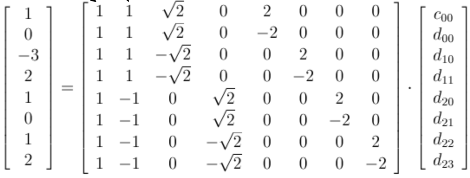
- Haar transform matrix \( H_n \)
- Discrete input vector \( v\in\mathbb{N}^{2^n} \)
- Wavelet coefficients \( b\in\mathbb{R}^{2^n} \)
- \( v = H_n \cdot b\equiv b=H_n^T\cdot v \) (\( H_n^T=H_n^{-1} \))
Matching
- Representation of Image is unique and contains location and intensity (due to orthonormal basis functions)
- Use first \( k \) wavelet coefficients that represent the image well enough
- Only represent broad structure of images
- Use Euclidean distance for matching
Multi-Resolution Analysis
- High resolution images:
- Have many pixels
- Wavelet transformation lead to high-dimensional equation systems
- Problem: Expensive
- Tilo: Not interested in details -> broad structure
- Solution: Fast wavelet transform
- Time complexity \( O(n) \)
- Algorithm works repeating the steps:
- Reduce resolution (leads to smaller equation systems)
- Store lost information to reconstruct images (provides the wavelet coefficients)
- Underlying technology: Multi-resolution Analysis
- Idea of MRA:
- Image in different resolutions without information loss
- Keep detail information but store it somewhere else
- Image signal consists of two parts: raster + detail
- Averaging and downsampling
- Summarize blocks of pixels (average color, remove noise)
- Average is the new pixel
- Works best for quadratic images (otherwise a single row or column must be stripped off, which is OK for MMDB purposes)
Formal
- \( V_k \): Original image
- Resolution stage \( k \)
- Works best for quadratic images \( 2^k \)
- \( V_{k-1} \): Raster of lower resolution (less pixels than \( V_k \))
- \( V_0 \): Single pixel (average color, not that helpful)
- Getting \( V_{i-1} \) from \( V_i \)
- Halve width/height iteratively by taking the average of two adjacent pixels (alternating width and height)
- Mean of pixels corresponding to \( V_i \)
- Store difference information
- Averaging and differencing
- Resolution state \( 0\leq i\leq k \)
- \( f_i(x,y) = f_{i-1}(x,y) + d_{i-1}(x,y) \)
- \( f_i \): Intensity of pixel \( p_i(x,y) \) in \( V_i \)
- \( d_i \): Detail (difference) information to reconstruct the pixel
- Reconstruct original image recursively:
- \( f_k(x,y) \)
- \( =f_{k-1}(x,y)+d_{k-1}(x,y) \)
- \( =f_{k-2}(x,y)+d_{k-2}(x,y)+d_{k-1}(x,y) \)
- \( =f_0(x,y)+\sum_{j=0}^{k-1}d_j(x,y) \)
- Additionally store matrix with difference between one of the pixels to the lower resolution image
- Advantage:
- No information loss
- Small differences
Filtering (Signal Processing)
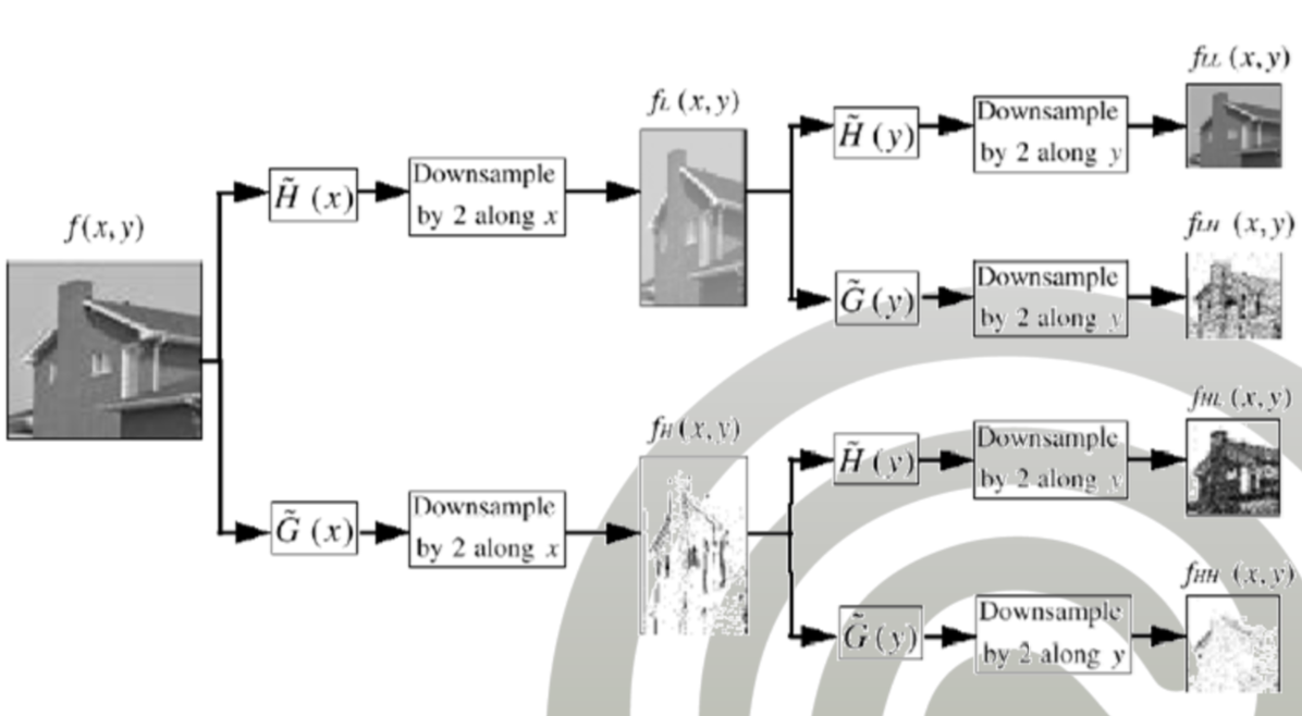
- Averaging and differencing corresponds to filtering
- High-pass filter
- Extracts detail information
- Baby-wavelets of higher order
- Shows changes
- Low-pass filter
- Extracts averages
- Baby-wavelets of lower-order
- Shows energy
- Application of filters:
LL, LH, HL, HH- H: High-pass (corresponds to differences)
- L: Low-pass (corresponds to average
HL: High-pass in X direction, Low-pass in Y direction, i.e., averages of the differences of X
- Feature array
- Save expected value + standard deviation of Wavelet coefficients
Shape-based Retrieval
Basics
- Shape
- Definition: A shape is the form of an object or its external boundary, outline, or external surface. (Wikipedia)
- Contribute significantly to similarity of images
- Often carry semantic information
- Often independent of color (e.g., banana shape may be red)
- Idea
- Simple shape-features: Round, elliptical, triangular, square, star, …
- Combine simple shape-features with other features (color, texture) to improve retrieval quality
- Fundamental problems
- Shape recognition/segmentation (which shapes are in an image)
- Semantic mapping (is it always possible?)
- Feature mapping/representation
- Similarity/comparison of shapes
Segmentation
- Task: Find relevant, displayed shapes in an image
- Problems:
- Relevance: Is water in background a relevant shape?
- What if the shape is not completely visible?, e.g., sunset
- What represents a shape?
- Is a shape homogeneous in color or texture? (e.g., Zebra, The Wave)
- Automated segmentation
- Hard problem
- Often specialized solutions for automated segmentation exist
- Shape-features removed from commercial systems (problems with segmentation)
- Segmentation in QBIC
- Seeded Region Growing
- Select seed points, add pixels to region if a certain criterion matches (e.g., gradient of greyscale)
- Problem: In QBIC this works only for monochrome surfaces
- What is a Shape?:
- Outline (outer perimeter) or the
- Area enclosed by the outline
- Approaches
- Area Detection: Areas with same brightness/color/texture
- Edge detection: Differences in brightness, gradient, watersheds
- Morphological operators: Filling (dilation/erosion)
- Active Contour: Segment the outline as closed curve
- Observation (personal): Most of the approaches should be combined to obtain a good segmentation. Remove noise with a Gaussian filter, then apply the edge-detection or threshold algorithm and improve the image with morphological operators.
Area Detection (Thresholding)
- Approach: Thresholding
- Used for grey value images
- Find area of shapes
- Idea
- Differentiate areas from background using brightness
- Assume that background is significantly darker/lighter than the foreground
- Can be combined with area-based approaches
- Split image in areas and detect objects in areas
- Use for colored images
- Assumption (deprecated)
- Thematically related areas have similar gray values
- Separate shape from background
- Approaches
- Fixed (static) threshold
- Fixed threshold for each image
- Good for similar lightning in all images
- Flexible (dynamic) threshold
- Depend on grey-value histogram
- Optional: Smooth histogram
- Fixed (static) threshold
- Algorithms
- ISODATA
- Ridler/Calvard, 1978
- Split histogram into two parts (divide mass of background and mass of object)
- Calculate two expected values
- Threshold is average of expected values
- Recursively compute expected values until no significant change
- Triangle algorithm
- Zack et al., 1977
- Connect highest peak with highest brightness value with a line
- Find maximal distance orthogonal to line
- Add certain constant –> This point is the threshold
- ==Why does this work? Why is this the threshold?==
- ISODATA
- Applications: Medical detection
- Advantage
- Simple
- Disadvantage
- Determination of right thresholds
- Assumption doubtful
- Strong color change of back- and foreground
- Does not work if object is enlightened (high and low brightness values)
- Decomposition of complex objects into simple shapes does not work
Edge detection
- Idea
- Find borders of objects
- Goal: Closed curves around object
- Maximum change in brightness function represents edge
- Brightness function
- \( I:\mathbb{N}\times\mathbb{N}\rightarrow [0,1] \)
- Idea: High change in brightness function (inflection point) represents edge
- Mathematical:
- Maximum/minimum in first derivative
- Zero/root in second derivative (real zero-crossing)
- Problem:
- Derivates require differentiable functions
- Image is discrete function
- Gradient calculation
- Estimate continuous function from complete image (e.g., Fourier transform)
- Estimate gradient of function from neighborhood (faster, e.g., Sobel filter)
- Approaches:
- Gradient-based method
- Laplacian Zero-Crossing
- Comparison
- Gradient: Shape is better (stronger) detected
- Zero-crossing: Noise is removed
- Both approaches may require the use of morphological operators
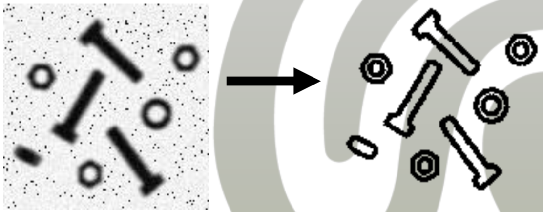
Gradient-based method
- Calculate magnitude of the gradient at each point
- e.g., using the Sobel filter
- If the gradient is high enough, the corresponding pixel belongs to an edge
- This approach is stricter than the Laplacian Zero-Crossing
- Then, use threshold algorithm for detection
- Avantage
- Simple filter
- Disadvantage
- Susceptible to noise (can be prevented by noise reduction pre-processing)
- Can not detect blurred/merging contours
Laplacian Zero-Crossing
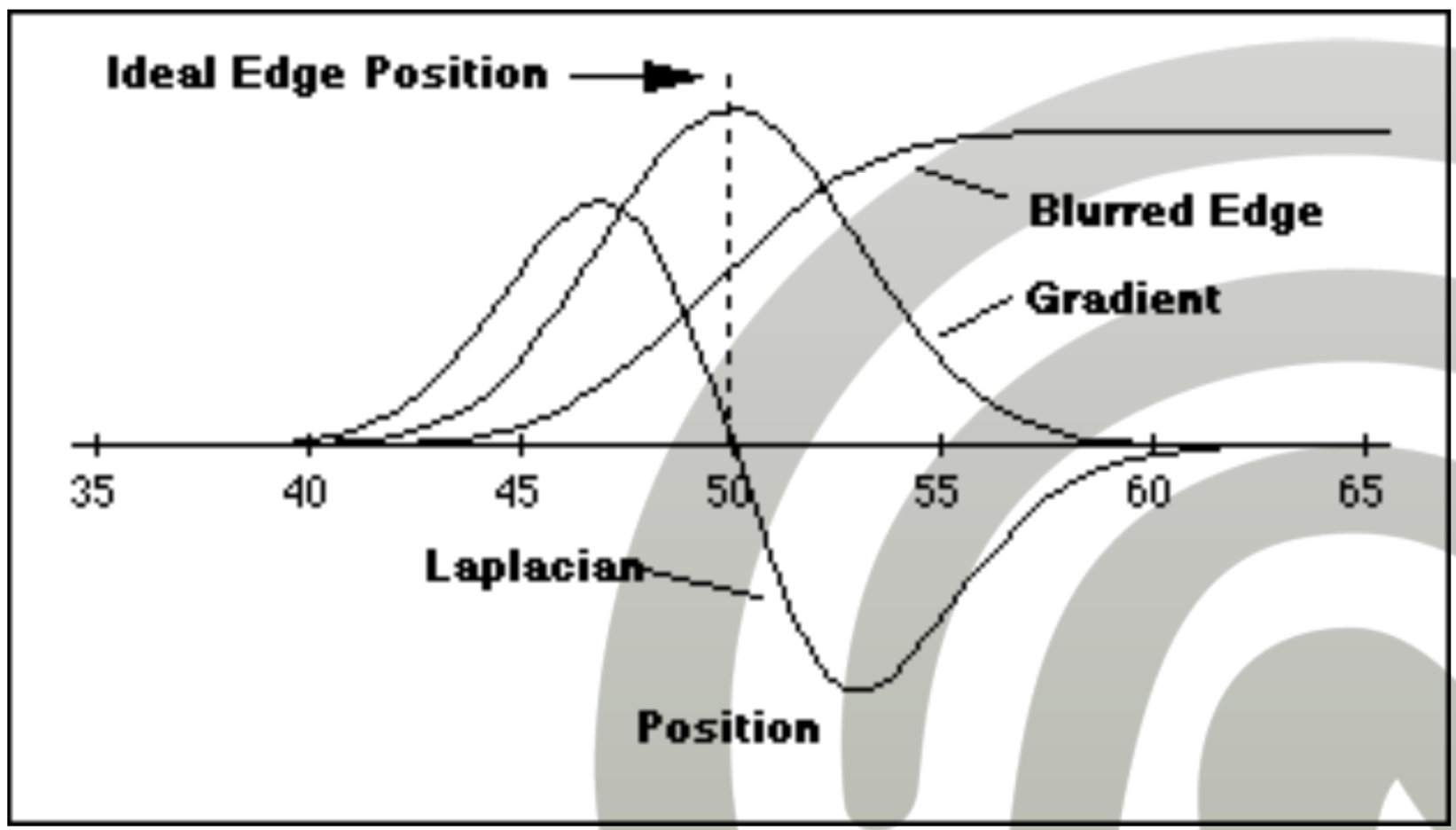
- Address problem of blurred edges and noisy images
- Zero-crossing of second derivative
- Idea:
- Zero passage of second derivate shows maximum gradient
- The ideal edge: Edges are only on real zero-crossings (not zero points)
- Creation of the new image:
- Pixels with real zero-crossings are marked (maybe multiplied by the magnitude of the gradient)
- Then, use thresholding to detect shapes
- Problem: Noise (apply Gaussian filter before)
Watersheds transformation
- What is a Watershed?
- A Watershed (dt. Wasserscheide) is a border between two adjacent rivers/seas.
- Assumption:
- Surfaces are defined by minimal grey values and zone of influence
- Area color of shapes is homogeneous (forming a lake)
- Idea:
- Flood a surface based on gray values
- Stop if gradient is too big
- Interpret the image as topological map
- Workflow
- Compute gradients of image
- Take minimal gradient(s) as markers or seed points (seed points may be set manually)
- Flood from each seed point
- If two floods meet, create a watershed line
- Advantage
- Enclosing/correct bordering
- Disadvantage
- Difficult to implement efficiently
- Over-segmentation
Active Contour
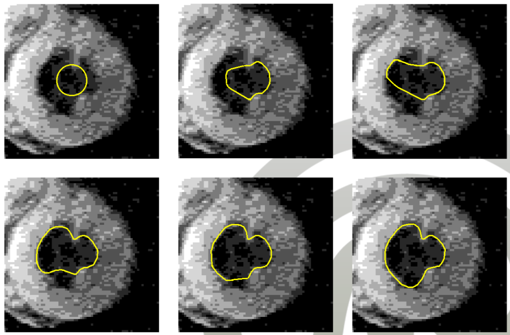
- Assumption:
- Regions are bordered/enclosed by closed curve (salient boundary)
- Regions are round/circle-like/elliptical
- Method
- A curve iterates towards the best possible separation
- Goal: Minimize energy
- Internal energy: Curvature/continuity
- External energy: Gradient of image (fit of curve)
- Advantage
- Can fit fuzzy edge
- Disadvantage
- The more accurate the contour should be, the more complex is the curve
- Initial curve must be given (usually manual given by seed point)
Morphological operators
- Problem: Noise
- Hard for shape segmentation
- May result in badly extracted shapes
- Goal: Easily recognize contours
- Idea: Morphological operations as pre-processing (remove noise, e.g., spikes in lines, holes in border)
- Binary neighborhood operations
- Change the surface
- Pixels are removed/added to edges
- Control operations using an operator mask (structure element)
- Workflow:
- Apply structure element to every pixels in source image
- Apply operator
- Structural element
- Define neighborhood around pixel (usually symmetrical but not required)
- Applied on each pixel, then apply operators
- Example: Symmetric areas of pixel
- Operators:
- Dilation (add pixels)
- Effect: Enlarge areas
- Connect objects with small distance, e.g., fill holes, blow up shapes
- e.g., add black pixel if any pixel in the structure element/neighborhood is colored
- Erosion (remove pixels)
- e.g., Add white pixel if any pixel in structure element/neighborhood is white
- Dilation (add pixels)
- Problem:
- Dilation and Erosion are not useful on their own
- Solution: Combine operations
- Operations:
- Opening
- Erosion followed by Dilation
- Eliminate small/thin objects
- Break tiny collections
- Smooth edges
- Closing
- Dilation followed by Erosion
- Fill small holes
- Join near objects
- Smooth edges
- Dilation followed by Erosion
- Opening
- Advantages
- Make it easier to obtain shapes
- Disadvantages
- Requires uniform grey values (either black or white pixels)
- Precise control is difficult
Representation
Basics
- Shape representation
- Per Object
- Contours (closed curve)
- Area (enclosed by curve)
- Hybrid (curve + surface)
- Per Image
- Describe all objects at once, i.e., the dominant edges in image (e.g., edge histogram)
- Per Object
- Shape similarity
- Interpretations
- Similar shaped objects
- Similar dominant shapes
- Choice is application-dependent
- Types:
- Contour-based (represent the outline)
- Area-based (represent the interior/area)
- Similarity measure
- Usually is complex
- Measure must be robust against:
- Shifts (translation invariance)
- Scaling (scale invariance)
- Rotation (rotational invariance)
- Interpretations
- Contour-based Retrieval
- Determine images with similarly shaped objects
- Outline is viewed as closed contour (result of the segmentation)
- Better semantics than global representation
- Area-based Retrieval
- Represent the contour and the interior of the shape
- High-level features (information-preserving)
- Hough / Walsh / Wavelet transforms
- Possible features:
- Low-level features
- Chain Codes (contour-based)
- Skeleton (area-based)
- Moments (area-based)
Low-Level Features
- Area non-information-preserving
- Contour-based
- Number of vertices
- Surface area (with holes)
- Enclosed area (without holes)
- Eccentricity (deviation from being circular, Wikipedia)
- Area-based
- Structural (primitive shapes covering an area)
- Geometric (Shape area, number of holes, compactness, symmetry, moments, moment invariants)
- Shape area (number of set pixels)
- Roundness (how close to circle)
- Euler number (Number of connected components - number of holes in component)
- Problem contour features:
- No scale invariance
- Shape is not reconstructable
- Shape similarity doubtful (e.g., number of vertices, area)
- Therefore: Combine with other features
Chain Codes
- Simple, pixel-based description
- Represent the contour of the shape
- Idea:
- Start with certain pixel
- Traverse contour clockwise/anti-clockwise
- Describe changes of edge direction (depend on predecessor pixel)
- Approaches:
- Freeman Code (Chain Code)
- Reduced Chain Code
- Reduce Difference Chain Code
- Shape Numbers
- Scale invariance:
- Improvement: Remove equal consecutive numbers
- Only for simple shapes
- e.g.,
000666222 -> 062
- Matching/similarity: Edit distance (e.g., Levensthein)
- Advantages
- Relatively easy (computationally + understandable)
- Disadvantage
- Scaling/rotation invariance very hard (does not work well)
- Lot of lost information
Freeman Code
- Freeman, 1961
- Direction codes (example)
- Right:
0 - Right-top:
1 - Top:
2 - etc.
- Right:
- Reduced Chain Code
- opposite direction gets same code
- e.g., Right/Left:
0, Top/Bottom:1
Reduced Difference Chain Code
- Base: Reduced Chain Code
- Motivation:
- Reduced Chain Code is rotation-dependent
- Long codes lead to expensive similarity computation
- Reduce Difference Chain Code (RDC)
- Summarize consecutive numbers to their difference
- Advantage: Compression
- e.g,
000222000 -> 00-200200 -> 0-2020
- Problem: Only works for rotations \( k*45° \)
Shape Numbers
- Bribiesca/Guzman, 1978
- Idea:
- Assign each type of edge a number
- Build a code for the shape
- Generate set of cyclic permutations of this code
- Sort permutations lexicographically
- Use first permutation as representation for shape
- Example codes:
- Convex corners
- Edges
- Concave corners
Levenstein Distance
- Part of family of edit distances
- String similarity measure
- \( A=(a_1,\ldots,a_n), B=(b_1,\ldots,b_m) \)
- Weighted Levenstein distance
- Idea: Convert string A to B using sequence of operations
- Operations
- Substitution (\( a\rightarrow b \))
- Insertion (\( \epsilon\rightarrow a \))
- Deletion (\( a \rightarrow\epsilon \))
- Operations have costs (natural number)
- Distance: Minimal cost for any sequence
- Advanced Levenstein distance
- Generalization of Levenstein Distance
- New operations:
- \( aab\rightarrow abb \)
- \( abb\rightarrow aab \)
- \( a\rightarrow aa \)
- \( aa\rightarrow a \)
Skeleton
- Blum, 1973
- Represent interior of the shape
- Skeleton:
- A thin version of a shape being equidistant to its boundaries
- Set of points (only the anchor points)
- Approaches
- Central axis:
- Number of centers of circles with maximum area, contained inside the shape
- Do not consider all centers (only the maximal ones)
- Symmetric boundary points
- Set of centers of bi-tangent circles
- Bi-tangent: Touch boundary in at least two points
- Sensitive to small changes
- Shock set (propagation model)
- Simulate waves from the borders
- Vertices are set where waves intersect
- Like Wildfire
- Central axis:
- Use skeleton graph for comparison
- Important: Consider holes
- Represent using a string
- Use disk with letters (like a segmentation of the space)
- Source: Shape recognition
- Matching:
- Similarity using an edit distance (e.g., Levenshtein)
- Operations
- Splice: Remove branch
- Contract: Represent \( n \) branches with a single node having \( n-1 \) branches
- Merge: Remove node between two skeleton branches
- Deform: Deform branch (Move node to another location)
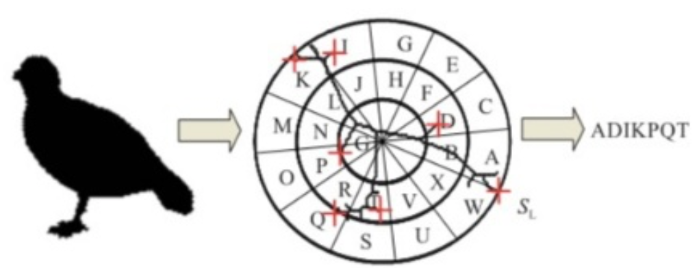
Moments
Stochastic foundation
- 1D discrete probability distribution \( f \)
- Finite set \( A \)
- \( \forall x\in A: f(x) \geq 0 \)
- \( \sum_{x\in A} f(x) = 1 \)
- Random variable \( X \) with distribution \( f \) (\( f(x) = P(X=x) \)
- Moment of X
- \( m_i = \sum_{x\in A} x^i \cdot f(x) \)
- First moment is expected value
- Central moments of X
- \( \mu_i = \sum_{x\in A} (x-m_1)^i \cdot f(x) \)
- First central moment is zero
- Second central moment is variance
- Property: Central moments are invariant to shifts
- 2D discrete probability distribution \( f \)
- \( f:A\times B \rightarrow [0,1] \)
- \( \forall (x,y) \in A\times B: f(x) \geq 0 \)
- \( \sum_{(x,y)\in A\times B} f(x,y) = 1 \)
- Random vector \( (X,Y) \) with distribution \( f \)
- Moment of (X,Y)
- \( m_{i,j} = \sum_{(x,y)\in A\times B} x^i \cdot y^i \cdot f(x,y) \)
- Central moment (X,Y)
- \( \mu_{i,j} = \sum_{(x,y)\in A\times B} (x-m_{1,0})^i \cdot (y-m_{0,1})^i \cdot f(x,y) \)
- \( \mu_{1,1} \) is covariance of X and Y
- Uniqueness theorem
- Each distribution function can be uniquely described by its moments
- Condition: All elements must exist (be finite)
Basics
- Idea:
- Use intensity function \( I \) to create probability distribution \( f_I \)
- Image moments: Moments of \( f_I \)
- Use image moments as features for the shape
- Normalize I to get probability distribution f
- \( f(x,y)=\frac{I(x,y)}{\sum_{(u,v) \in A\times B} I(u,v)} \)
- Uniqueness theorem:
- Moments of \( f_I \) (image moments) are an information-preserving description
- Use first \( k \) image moments as features (low-level)
- Translation invariance:
- Use central moments
- Scaling invariance:
- Use normalized central moments
- \( \eta_{i,j} = \frac{\mu_{i,j}}{(\sum_{(x,y)\in A\times B} I(x,y))^{(i+j)/2}} \)
- Rotational invariance:
- Idea:
- Rotation/scaling in \( \mathbb{R}^2 \) are linear transformations
- Rotation by \( \alpha \) and scaling by \( s \): \( A = s \cdot (\begin{smallmatrix}\cos(\alpha)& -\sin(\alpha)\\ \sin(\alpha) & \cos(\alpha)\end{smallmatrix}) \)
- Intensity function of shape yields distribution \( f \)
- Distribution \( f \) yields normalized central moments \( \eta \)
- Goal:
- Shape A is linearly transformed to shape B, the normalized central moments of A and B should be invariant under the new function \( g \)
- Invariant function \( g \)
- \( g(\eta_{0,0},\eta_{0,1},...)=g(\eta_{0,0}',\eta_{0,1}',...) \)
- \( g \) transforms normalized central moments to new characteristic values so that rotation does not change these values
- Idea:
Moment Invariants
- Hu, 1962
- Moment Invariants: Metrics that are translation, scaling and rotational invariant
- Algebraic invariants
- Definition
- \( g:\mathbb{R}^n \rightarrow \mathbb{R}^n \)
- Weight \( w\in \mathbb{R} \)
- Matrix \( A\in\mathbb{R}^{n \times n} \) with full rank
- \( g \) is relative invariant with weight \( w \) if for all matrices \( A \) and all \( x\in\mathbb{R}^n \): \( g(Ax)=det(A)^w \cdot g(x) \)
- Absolute invariant: \( w=0 \)
- Important Property
- \( g_1, g_2 \) are independent with weights \( w_1, w_2 \)
- \( h(x) = \frac{g_1(x)^{w_2}}{g_2(x)^{w_1}} \)
- \( h \) is absolute invariant (\( h(Ax)=h(x) \))
- Important: Independent of \( A \) (rotation does not matter)
- Definition
- Hu propose seven absolute moment invariants - \( g_1(\ldots)=\eta_{0,2}+\eta_{2,0} \) - \( g_2(\ldots)=(\eta_{0,2}+\eta_{2,0})^2+4\eta_{1,1}^2 \) - …
- Similarity
- Use vector of characteristic values (result of invariant functions)
- Euclidean distance
- Separability property
- How many moment invariants do we need?
- Two different shapes must differ in at least one component
- Two similar shapes have same equal/similar components
- Use property to estimate number of invariants
- Improvement
- Use other types of moments
- Zernike moment
- Tschebyschew moment
- Fourier moment
- Simplified computation special shapes:
- Splines (polynomial functions)
- Polygons
- Curves (parametric representation)
- Use other types of moments
- Experiments
- Hu, 1962
- STAR (Mehtre et al, 1995)
- Company logos
- Average retrieval efficiency (probably F1) of 85% - 88%
- In combination with other features 89% - 94%
Discrete Image Correspondence
- Method for testing image similarity
- Advantages
- Simple
- Fast
- Steps
- Detect points of interest
- Describe neighborhood of points of interest (using vectors)
- Match description vectors
- Points of interest
- Capture distinctive locations (==How to get them???==)
- Scale/rotation invariant
- Algorithms
- SIFT
- SURF
- Matching
- Distance measure on feature vector (e.g., Mahalanobis, Euclidean)
- Advantage
- Easy
- Scale/rotation/lighting/contrast invariant
- Suitable fir searching similar images
- Disadvantage
- No detailed information
- Bad for querying objects
SIFT
- Scale-invariant feature transform
- Multi-resolution analysis
- Uses linear Gaussian low-pass filter
- Detection:
- Filter image
- Features are extreme points in gray-level histogram
- Stable point
- Extreme points in several consecutive resolutions
- Are scale invariant
- Only keep stable points
- Description
- Interest points get an orientation
- Orientation based on grey-level histogram in direction of change
- ==Peaks???==
- 36 directions
- Feature vector: 160 orientations
SURF
- Speeded Up Robust Features
- Detection
- Box filter (averaging, better performance)
- Consider consecutive resolutions
- Description
- Circular neighborhood (==Why?==)
- Haar wavelets