Video Retrieval

Basics

• Motivation:
  • Video is important medium
  • e.g., clips, presentations/lectures, conferences, news, entertainment
  • News: Detect interesting clips
  • Entertainment: Genre detection, Advertisement detection
• Basic Requirements:
  • Store, access, recover video
  • Scalability
• Challenges:
  • Video is continuous medium
    • Contains audio stream, image stream, subtitles
  • Organization
    • Structured in time and space
    • Video is document (semantic; not a set of frames)
    • Video abstraction: Decompose it into semantic, structured parts (e.g., storyboard)
• Retrieval result:
  • Set of video abstractions
  • Summary sequence: Overview of content (e.g., keyframes)
  • Video highlight: Scenes from a video (e.g., trailer)
  • see Video Abstraction

Commercial Databases

• BLOBs, Smart BLOBs
• Metadata retrieval
• Key-frame-splitting
• Features:
  • Retrieve data
  • Define data types/functions
  • Secure/recover video data
  • Import/export clips
  • Store/maintain video attributes
  • Play video
  • Support a variety of video formats
• No content-based retrieval :(

Retrieval Techniques and Features

• Text Retrieval
• Audio Retrieval
  • Voice detection (for an actor)
• Image Retrieval
  • Detection of subtitles
  • Classification of objects (also movements)
  • Person/object recognition/segmentation
• Movement recognition (direction and speed)
  • Temporal behavior of objects
  • e.g., edge detection and comparison between frames
  • MPEG-4 Extraction of moving objects (use for compression)
• Camera movement recognition
  • Changes of camera angle, zooming, fading
  • Detect effects
• Time-place-relationships
  • Trajectories and crossings
  • e.g., car accidents by observed crossings

---

Video Abstraction

• Goal: Create temporal/spatial structuring of content
  • Compare to abstract for texts (however, video abstracts are more general than text abstracts)
  • e.g., objects falling down
• Sub-domains:
  • Video modeling/representation
  • Video summary (still)
  • Video skimming (moving)
    • Video highlighting
• Automatic Video Abstraction
  • Manual editing is not possible
  • Purpose: User can determine relevance
  • Advantage: Save transmission time / bandwidth (videos are usually not on local system)
• Video modeling/structure
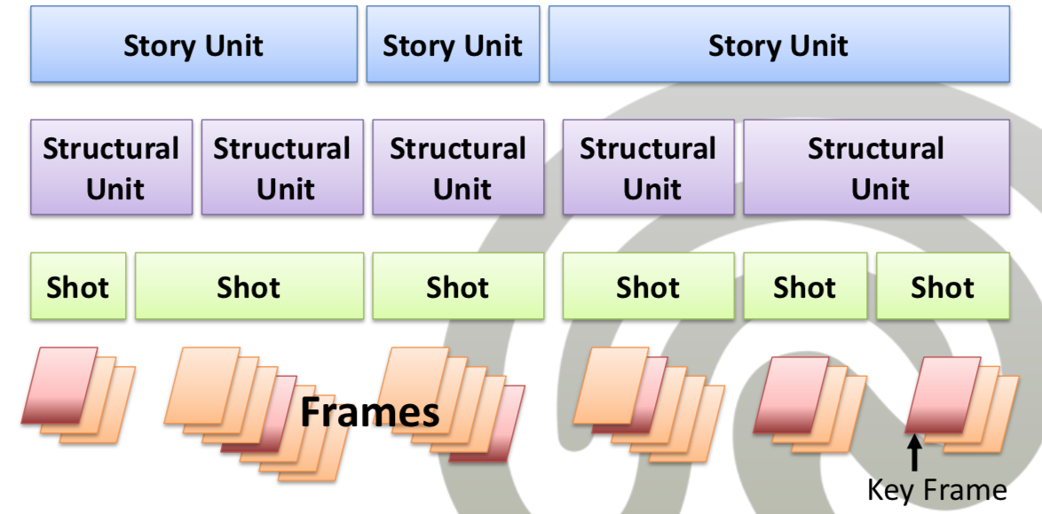
  • Story unit
    • High-level, semantic unit
  • Structural units
    • Semantic unit
    • e.g., introduction, problem statement
  • Shots:
    • Action a camera takes
  • Frames:
    • Adjacent frames are assumed to be similar
  • Key frame: Anchor showing what happens in a scene/typical frame
• Example: News broadcast
  • Story unit: War in Iraq
  • Structural: Introduction, transmission, summary
  • Shorts: Anchorman, pan of desert, bombing a city, refugees

Result Presentation

• Result presentation
  • Text: Summary, abstract, snippets of documents
  • Image: Thumbnails of results (reduced resolution)
  • Audio: Earcon, short snippet
  • Video: How to present results?
• Requirements:
  • Minimize amount of data (do not play complete video)
  • Assessment of relevance (do not show irrelevant parts)
  • No textual summary (Show images/play audio)
• State-of-the-art approaches:
  • Thumbnails: Yahoo video
  • Play parts of video: Bing, Youtube
  • Video structure (shots/keyframes): videosurf.com
• Other approach: Video abstract(ion)

Video Summary

• Definition
  • Like a storyboard (static)
  • Order keyframes of shots and annotate with characteristic audio
  • Still summary
• Idea:
  • Represent mostly each shot
  • Should contain all essential parts
    • Sampling of entire video
    • Key frames can be selected
• Summary based on shots
• Important: Order of frames should be kept (better understanding)

Keyframe Selection

• Goal: Select keyframe from a shot
• Average color
• Random
• First/middle/last frame

Keyframe Composition

• Goal: Select keyframes for the summary
• Keyframes only (simple)
  • Use key frames of all shots in chronological order
  • Problem: Often, too many key frames (e.g., fast cut scenes in advertisement)
• Difference-based selection
  • Choose first show (e.g., contains title)
  • Compare two consecutive key frames
  • If the difference exceeds a threshold, use second key frame for summary
• Cluster-based selection
  • Cluster all keyframes
  • Select one key frame per cluster
  • Clustering method:
    • Complete-linkage clustering
    • Partition clustering
  • Important: Keep order of frames

Audio Information

• Goal:
  • Select most important sentence of shot
  • Annotate keyframe with this sentence
  • e.g., “I’m Iron Man”
• Requirement:
  • Speech-to-text or
  • Subtitles with time codes
• Method: LSA
  • Document: Each sentence
  • Build term-sentence matrix
  • Perform Latent Semantic Indexing (clustering)
  • Axis correspond to topics (linear combination of terms)
  • Personal idea: Choose sentence for a shot which is most discriminatory for its topic

Video Skimming

• Also called summary sequence
  • Short (a skim of the video)
• Goal:
  • Provide overall impression of entire video in small time
  • Moving summary
  • Dramatically shortened duration
  • Important: Scenic structure of video (story unit)
• Important aspects/questions:
  • Duration to comprehend contents of a scene (e.g., close-up with emotions)
  • Impact of scene ordering on understandability (syntax of video)

Approaches

• Uniform temporal scaling
  • Shorten video uniformly
  • e.g. remove every second frame
  • Problem: Not all shorts are equally important
  • Better:
    • Drop whole shots (e.g., Non-uniform skimming)
    • Use story units (e.g., Video Highlighting)
• Automatic video summaries
  • Informedia project
    • Automatic speech recognition
    • Still, error-prone
  • Steps
    • Estimate visual complexity of shots
      • Time to understand shots
      • Using psychological experiments (Sundaram/Chang, 2002)
    • Use film theory to select important scenic structures
  • Advantage: Compression about 80 % is possible

Video Highlighting

• Goal:
  • Transfer atmosphere of movie and arouse interest
  • Select important scenes (do not summarize entire video)
  • Focus on story unit
  • Do not show the end
  • e.g., trailer
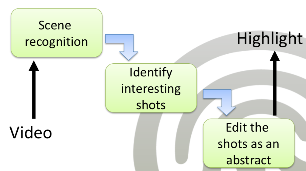
• Procedure (schematic overview)
  1. Video segmentation
     • Detect shots/scenes
  2. Video analysis
     • Scene recognition
     • Analyze text/effects/close-ups
  3. Clip selection / Highlight generation
     • Special effects?
     • Which clips to include?
  4. Clip combination / Video editing
     • Maintain order? cutting type? audio track?
• High-quality abstracts / Requirements:
  • According to Film theory
  • Contain these components/scenes:
    • Relevant entities/individuals (high contrast, e.g., black scene, white dress)
    • Actions (strong movement)
    • Mood (variation from average color distribution)
    • Dialogue (close-up faces + audio)

Video Analysis

• Task:
  • Analyze shots
  • Group shots (scenes, semantic units)
  • Called scene detection
• Scene Detection
  • Use face detection for actors and dialog
  • Use text extraction for title and subtitles
  • Use special effects recognition for interest
  • Heuristics
    • Common background (significant change between scenes)
    • Alignment of video- and audio-cuts (cut in video without cut in audio is usually the same scene)
    • Dialogues (present in a scene)
      • Close-ups shot: At least 30 % of area is face (usually dialogs)
    • Important people appear often (remove frames with un-important/rarely-occurring actors)
• Face detection
  • Rowley et al., 1995
  • Idea:
    • Training of neural networks with given salient points (position of eyes/nose)
  • Improvement:
    • Color Filter: Filter frames with dominant skin color (pre-selection of frames)
    • Group similar faces: Similar distance between salient points
• Text Extraction
  • Goal:
    • Movie title should be in abstract
    • Text in video has a meaning
  • Detect text regions (high contrast, contiguous region, low color variance, across several frames)
  • Cluster into rows (using vertical/horizontal size and distance)
  • Use OCR to convert to text
  • Title has largest font size
  • Drawback: Only for stationary/linearly moving text
• Special effects recognition
  • e.g., explosions, gunfire
  • Classification of effects:
    • Pfeiffer et al., 2001
  • Goal: Integrate into abstract (for interest)
  • Use audio track for detection
    • Loudness, frequencies, pitch
    • e.g., peaks, detect acoustic events

Highlight Generation / Clip Selection

• Task: Select clips for highlight
• Parameters:
  • Goal length (controls selection criteria) or
  • Thresholds for criteria (e.g., which scenes to include, effects, faces, …)
  • Results in knapsack problem
• Workflow
  • Choose Scene candidates
  • For each scene, choose a Shot candidate
    • Whole scene is too long
    • Even ratio of dialogue and action shots
    • No scenes from the end
  • Create video (using video and audio editing)
• Scene candidate:
  • Text sequences (e.g., title text)
  • Dialogues / close-ups
  • Special effects
• Shot candidate:
  • Action-rich shots (use motion vectors)
  • Shots with average color distribution of video
  • Fitting genre
    • Using automatic genre detection
    • Typical parameters of the genre
    • e.g., action

Video Editing

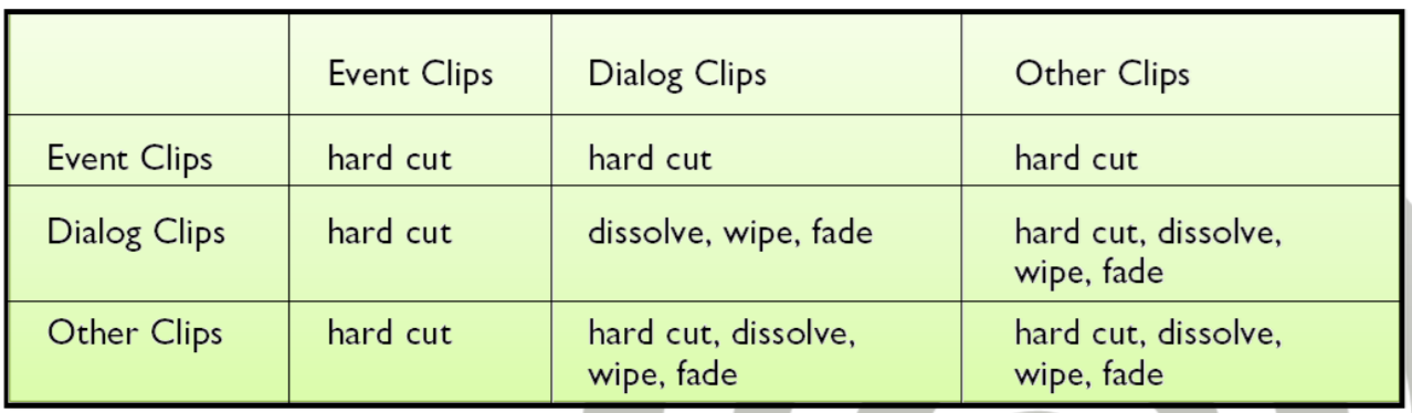
• Goal: Combine shot candidates to the final video
• Options:
  • Keep order of shots
    • Important for understanding
    • A trailer may deviate from original order (must be well-considered)
    • Semantic decision (usually, keep original order)
  • Type of cuts
    • Hard cut: Strong separation (e.g., action vs. environment)
    • Soft cut: Text/dialogue/fill-up scenes
• Audio Editing
  • Problem: Audio can not be abbreviated
  • Approaches:
    • Keep audio events of special effects (boom)
    • Ignore audio of filler scenes
    • Dialogs: Audio cut has priority (show complete dialogue scene)
  • Background audio track (e.g., soundtrack)

---

Video Similarity

• Use cases:
  • Ranking
  • Duplicate detection
    • e.g., videos having different resolution
  • Copyright infringement detection
  • Indexing/similarity efficiency (requires similarity measure)
• Measures
  • Idea: Percentage of similar frames
    • Compare to Tanimoto similarity for texts (Jaccard Index)
    • Problem: No timing behavior/perception
  • Idea: Detect audio-visual features of shots
    • e.g., color distribution, motion
    • Use shots for efficiency reasons (instead of frames)
• Trade-off:
  • Accuracy (number of features) vs. efficiency
  • Efficiency more important than accuracy
• Definition Near-duplicate videos
  • Wu/Ngu/Hauptmann, 2006
  • Two identical videos may differ in:
    • File formats
    • Encoding parameters
    • Photometric variations (color, lightning)
    • Editing operations (caption, logo)
    • Different length

Signatures

• Idea:
  • Select small number of features representing a video with minimal errors
  • Minimize distance between video and representation (e.g., k-means, k-medoids)
• Assumptions:
  • Each frame represented in metric space \( F \)
  • Feature space has metric \( d \)
  • Consider shot as cluster of feature vectors
    • Keyframe of shot is representative feature vector
  • Similarity independent of ordering of shots (only visual/perceptional similarity)
  • Video: Finite, unordered set of feature vectors
• Distance measure \( d \):
  • Dissimilarity measure
  • Approach Cheung/Zakhor, 2003
    • Use threshold \( \epsilon>0 \)
    • \( x \) and \( y \) are similar iff \( d(x,y)\leq \epsilon \)

Naive Video Similarity

• Basic idea: Percentage of similar frames
• Idea:
  • Number of frames of video \( X \) having at least one similar frame in video \( Y \) and vice versa
  • Divided by number of frames of \( X \) and \( Y \)
• Formal:
  • \( nvs(X,Y,\epsilon)=\frac{1}{|X|+|Y|}(\sum_{x\in X} 1_{\{y\in Y: d(x,y)\leq\epsilon\}}+\sum_{y\in Y} 1_{\{x\in X: d(x,y)\leq\epsilon\}}) \)
  • \( 1_A= 1 \iff A\neq\emptyset \) (otherwise 0)
• Problem: Un-intuitive
  • \( Y \) contains visually similar frames of \( X \)
  • \( |Y|>>|X|\rightarrow nvs(X,Y,\epsilon)\approx 1 \)
  • Example:
    • \( X \) contains two dissimilar frames
    • \( Y \) contains 8 similar frames to the first frame of \( X \)
    • \( nvs(X,Y,\epsilon)=0.9 \)
    • Instead, it should be \( 0.5 \)
• Solution: Clustering
  • Cluster frames with radius \( \epsilon \)
  • \( x,y\in X \) belong to same cluster iff \( d(x,y)\leq\epsilon \)
  • Single-linkage clustering:
    • Connected components in a \( d<\epsilon \)-graph
    • Problem:
      • Degeneration of clusters
      • Visual similarity is not transitive (\( x,y,z \))
      • \( x \) and \( z \) can be similar to \( y \) but un-similar to each other
      • In videos, there often is small change between shots
  • Solution: \( \epsilon \) compact cluster (Ideal Video Similarity)

Ideal Video Similarity

• Definition: \( \epsilon \) compact cluster
  • All elements in cluster have at most distance \( \epsilon \) to each other
  • Clustering \( [X\cup Y]_\epsilon \) contains clusters of \( X \) and \( Y \)
  • If a cluster contains frames from \( X \) and \( Y \), they are visually similar
  • Leads to Ideal Video Similarity
• Idea:
  • Jaccard index
  • Percentage of \( \epsilon \)-compact clusters containing frames from both videos relative to all clusters
• \( ivs(X,Y,\epsilon)=\frac{1}{|[X\cup Y]_\epsilon|}\sum_{C\in[X\cup Y]_{\epsilon}} 1_{C\cap X}\cdot 1_{C\cap Y} \)
• Mixed cluster: Cluster containing frames from both videos
• Pure cluster: Cluster containing frames from only one video
• Naive Calculation
  • \( |X|\cdot|Y| \) distance calculations
• Samling Calculation:
  • Randomly select \( m \) frames per video
  • Calculate \( ivs \) based on the samples
  • \( W_m \): Similar pairs from the samples
  • Advantage: Efficient computation
  • Disadvantage: Worse results
  • How many samples \( m \)?
    • Scenario: \( X \) and \( Y \) are identical (\( ivs=1 \))
    • Expected value of number of similar pairs: \( E(W_m)=\frac{m^2}{|X|} \)
    • Find at least one similar pair: \( m=\sqrt{|X|} \)
• Problem: Very bad
  • Does not work
  • \( m=\sqrt{|X|} \) only leads to a single similar pair
  • Leads to \( d(X,Y)=\frac{E(W_m)}{m}=\frac{1}{\sqrt{|X|}} \)

Voronoi Video Similarity

Voronoi Tessalation

• Decomposition of metric space into disjoint parts
• Formally
  • Metric space \( (F, d) \)
  • Discrete points \( X\subseteq F \)
  • Task: Divide F in |X| disjoint parts
• Tessellation: Each point from a \( x_i\in X \) region is closest point to \( x_i \)

Basics

• Idea:
  • Build Voronoi tessalation with the keyframes of the video
• Voronoi Tesselation
  • Feature space \( F \)
  • \( X=\{x_t:t=1,\ldots,l\} \) (\( l \) frames)
  • \( V(X) \): Voronoi diagram
  • Voronoi cell \( V_X(x_t) \) contains all feature vectors which are more similar to \( x_t \)
  • Compare frame only to \( x_t \)
• Cluster of frames:
  • Combine Voronoi cells (union)
  • \( V_X(C)=\bigcup_{x\in C} V_X(x) \)

Similar Voronoi Regions

• Idea: Intersect Voronoi cells if their feature vectors are similar
• \( R(X,Y,\epsilon)=\bigcup_{d(x,y)\leq\epsilon} V_X(x)\cap V_Y(y) \)
• Volume of \( R \) is a similarity measure for videos
• Problems:
  • Finite space (no problem finite number of vectors)
  • Lebesgue integral (volume must be measurable)
  • Normalization (\( Vol(F)=1 \))

Voronoi Video Similarity

• \( vss(X,Y,\epsilon) = Vol(R(X,Y,\epsilon)) \)
• \( =Vol(\bigcup_{d(x,y)\leq\epsilon} V_X(x)\cap V_Y(y)) \)
• \( =\sum_{d(x,y)\leq\epsilon} Vol(V_X(x)\cap V_Y(y)) \)
• Informal, this is the ratio of the intersections of the Voronoi cells
• Important: Voronoi vectors must be similar to at least \( \epsilon \)

Estimation

• Goal:
  • Estimate Voronoi video similarity (VSS) due to hard computation
• Estimate using the Basic Video Signature Similarity
• Problem:
  • Comparing every frame from \( X \) with the corresponding frame from \( Y \) is too expensive
  • Solution: Distribute seed points
• Two types:
  • Random sampling over \( F \)
  • Random sampling over the Voronoi cells

Basic Video Signature Similarity

• Idea:
  • Generate \( m \) seed vectors \( s_1,\ldots,s_m \)
  • Similarity measure:
    • Use the percentage of seed vectors being in \( R(X,Y,\epsilon) \)
    • Note: \( s_i\in R(X,Y,\epsilon) \iff d(g_X(s_i),g_Y(s_i))\leq\epsilon \)
    • For each seed, check if it is in \( R \)
• Video signature:
  • Video \( X \), \( m \) samples
  • \( g_X(s_i) \): Frame closest to \( s_i \)
  • \( X_S=(g_X(s_1),\ldots,g_X(s_m)) \)
• Basic Video Signature Similarity
  • \( vss_b \) (Degree of overlap)
  • Probability event \( s\in R(X,Y,\epsilon) \) represents volume of \( R(X,Y,\epsilon) \)
  • \( vss_b(X_S,Y_S;\epsilon,m)=\frac{\sum_{i=1}^m 1_{d(g_X(s_i),g_Y(s_i)\leq\epsilon}}{m} \)
  • \( vss_b \) is an estimator for \( vvs \)
  • Use identical seeds for a complete collection
• Trade-off: Signature length \( m \)
  • Retrieval quality vs. efficiency

Random Sampling over \( F \)

• Independent and uniformly distributed over \( F \)
• Estimate Error Probability
  • Given:
    • Video database \( \Lambda \) with \( n \) videos
    • \( m \) seeds
    • Constant \( \gamma>0 \) (maximum deviation)
  • \( P_{err}(m)=P(\sum_{X,Y\in\Lambda} |vss(X,Y,\epsilon)-vss_b(X_S,Y_S,\epsilon,m)|>\gamma) \)
  • Guarantee \( P_{err}(m)\leq \delta \)
    • \( \delta \) is chosen constant
    • \( m\geq \frac{2\ln n-\ln \delta}{2\gamma^2} \)
    • Logarithmic bound w.r.t. to size of the video collection \( n \)
  • Proof:
    • Hoeffding’s inequality
      • Describes Probability that a sum of independent random variables differs at most c from their expected values
      • Random variables \( X_1,\ldots,X_n \) with \( a_i\leq X_i-EX_i\leq b_i \) (almost sure)
      • Constant \( c>0 \)
      • \( P(\sum_i (X_i-EX_i)\geq c) = \leq exp(\frac{-2c^2}{\sum (b_i-a_i)^2}) \)
    • \( \rho(X,Y) = vss(X,Y; \epsilon) \)
    • \( \hat{\rho}(X,Y) = vss_b(X_S,Y_S; \epsilon, m) \)
    • \( P(|\rho(X,Y)-\hat{\rho}(X,Y)|> \gamma)\leq 2\exp(-2\gamma^2m) \)

Random Sampling over Cells

• Problem: \( VSS \) is not always \( IVS \)
  • \( VSS \) is \( IVS \) if clusters are evenly distributed over entire space (Voronoi cells have equal size)
  • Estimation should depend on Voronoi cell size
  • Hitting a Voronoi cell should be equally probable
• Goal: Estimate \( ivs \) using \( vss_b \)
• Idea: Distribute seeds evenly over Voronoi cells (not space)
• Density function:
  • Videos \( X, Y \)
  • Density at \( u\in F \):
    • \( C\in [X\cup Y]_\epsilon \)
    • \( u\in V_{X\cup Y}(C) \)
    • \( f(u, X\cup Y)=\frac{1}{|[X\cup Y]_\epsilon|}\cdot\frac{1}{Vol(V_{X\cup Y}(C))} \)
  • \( f \) inversely proportional to volume of cell (large cell – small density)
  • \( f \) is constant within the Voronoi cell of each cluster (uniform within each cluster)
• Generation of seeds:
  • Choose a cluster (uniformly distributed)
  • Choose random point within the cluster (uniformly distributed)
  • Assumption:
    • Only holds for seed generation for a pair of videos
    • Clusters \( c_X\in [X]_{\epsilon} \) and \( c_Y\in[Y]_{\epsilon} \) are either identical (\( d(c_X,c_Y)\leq \epsilon \)) or apart (\( d(c_X,c_Y)>\epsilon \))
  • \( ivs(X,Y,\epsilon)=\sum_{d(x,y)\leq\epsilon} \int_{V_X(x)\cap V_Y(y)} f(u; X\cup Y)du \)
    • \( =\sum_{C\in[X]_{\epsilon}\cap[Y]_{\epsilon}} \int_{V_{X\cup Y}(C)} f(u; X\cup Y)du \)
    • \( =\sum_{C\in[X]_{\epsilon}\cap[Y]_{\epsilon}} \int_{V_{X\cup Y}(C)} (\frac{1}{|[X\cup Y]_\epsilon|}\cdot\frac{1}{Vol(V_{X\cup Y}(C))})du \)
    • \( =\frac{1}{|[X\cup Y]_\epsilon|}\cdot\sum_{C\in[X]_{\epsilon}\cap[Y]_{\epsilon}} \frac{1}{Vol(V_{X\cup Y}(C))} \int_{V_{X\cup Y}(C)} 1 du \)
    • \( =\frac{1}{|[X\cup Y]_\epsilon|}\cdot\sum_{C\in[X]_{\epsilon}\cap[Y]_{\epsilon}} \frac{Vol(V_{X\cup Y}(C)}{Vol(V_{X\cup Y}(C))} \)
    • \( =\frac{|[X]_\epsilon\cap[Y]_\epsilon|}{|[X\cup Y]_\epsilon|} \)
  • Jaccard index (Definition of the IVS)

Application

• Problem:
  • Density function \( f \) depends a specific pair of videos \( X \) and \( Y \)
  • Find density function working for the whole collection
  • For collections, we require same seeds
• Idea:
  • Use representative training set to define the collection-dependent density function
• Training algorithm:
  • Given:
    • \( \epsilon_{SV} \)
    • Representative training set \( T \) (containing frames)
  • Steps (repeat \( m \) times):
    1. Identify all clusters \( [T]_{\epsilon_{SV}} \) for \( T \)
    2. Choose any cluster \( C\in[T]_{\epsilon_{SV}} \)
    3. Create a seed in the Voronoi cell of \( C \)
       • Either generate random vectors until one is in \( V_T(C) \)
       • Or use random frame from \( C \)
• Experiment
  • 15 videos from MPEG-7 content set
  • Avg. length: 30 min

Voronoi Gap

• Problem:
  • \( VVS \) and \( IVS \) are only the same if clusters are either identical or clearly separation
  • Feature vectors are approximation of visual perception
  • Voronoi cells may diverge a little bit
  • \( VVS \) under-estimates the \( IVS \)
    • Videos may be visually similar but this is not recognized
    • Dissimilar video signatures (although videos are similar)
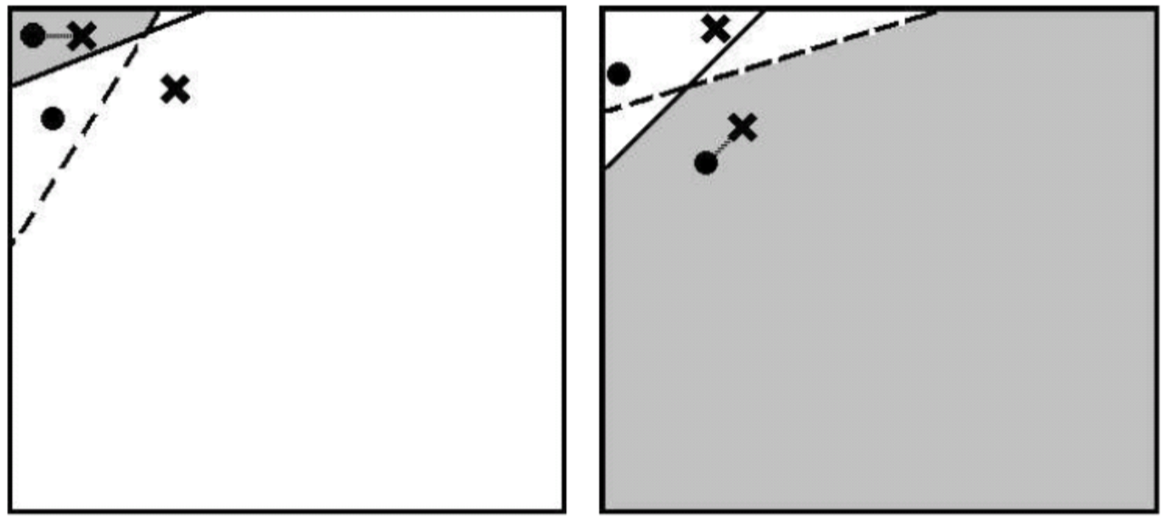
• Definition Voronoi Gap
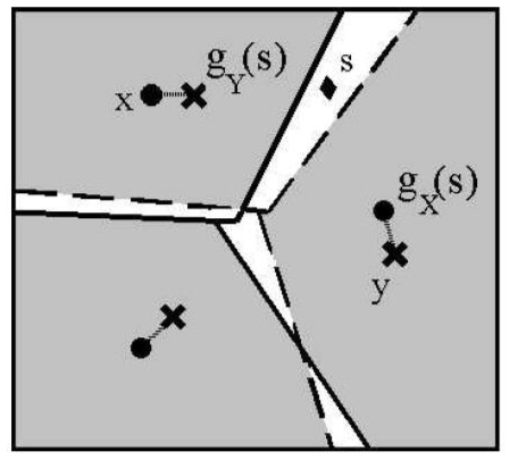
  • Voronoi Gap \( G(X,Y,\epsilon) \)
  • \( G=\{s\in F\mid d(g_X(s),g_Y(s))>\epsilon\} \)
  • \( \exists x\in X: d(x, g_Y(s))\leq\epsilon \)
  • \( \exists y\in Y: d(y, g_X(s))\leq\epsilon \)
• Voronoi Gaps must be considered
• Goal:
  • Avoid seed vectors lying in the Voronoi gap
  • Seed vectors should be away from the border
• Solution: Change generation
  • How to find seed vectors being in the Gap?
  • Definition of Gap does not help: Requires calculation
  • Observation:
    • Equidistance pair of frames for Voronoi Gap member \( s \)
    • \( d(x, g_X(s))\approx d(y, g_Y(s)) \) but
    • \( d(x, g_X(s))>\epsilon \)
    • \( d(y, g_Y(s))>\epsilon \)
  • Criterion:
    • For every seed \( s \) in the Voronoi Gap, there is a \( x\in X \): \( d(x, g_X(s))>\epsilon \)
    • \( d(x,s)-d(g_X(s),s)\leq 2\epsilon \)
  • Test:
    • If no vector \( x\in X \) with \( d(x, g_X(s))>\epsilon \) and \( d((x,s)-d(g_X(s),s)\leq 2\epsilon \)
    • Then \( s \) is never in the Voronoi Gap between \( X \) and any other video
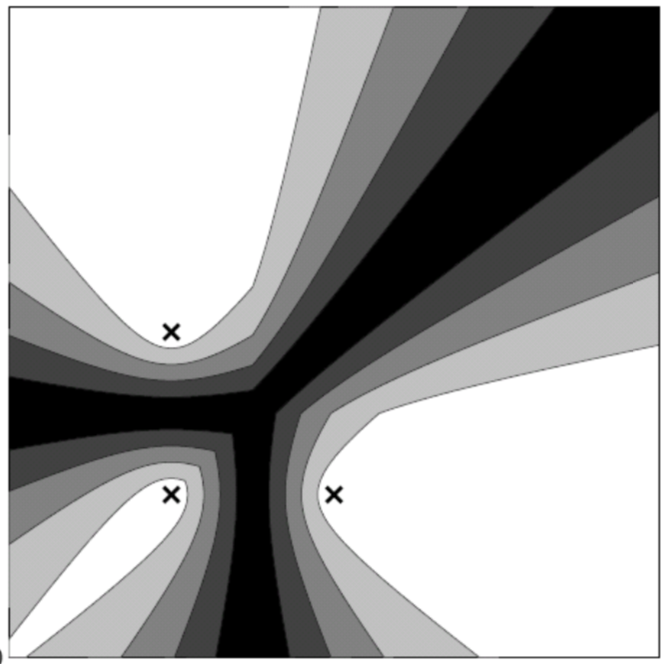
• Ranking function \( Q \)
  • \( Q(g_X(s))=\min_{x\in X, d(x, g_X(s))>\epsilon} d(x,s)-d(g_X(s),s) \)
  • Distance between seed and borders of cells

Application

• Safe seeds have \( Q>2\epsilon \) (safe = not in a Voronoi Gap)
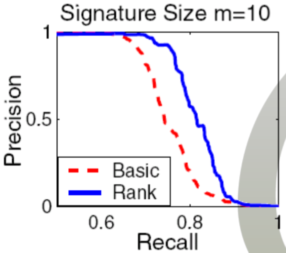
• Ranked Video Similarity \( vss_r \)
• Symmetric \( vss_r \)
  • Symmetrical \( vss_r \) between two videos is defined by the seeds with the highest ranking in \( X_S \) and \( Y_S \)
  • \( m \) number of frames (generate more seed vectors)
  • \( vss_r(X_S,Y_S;\epsilon,m)=\frac{1}{m}(\sum_{i=1}^{m/2} 1_{d(g_X(s_{j[i]}, g_Y(s_{j[i]}) \leq \epsilon} + \sum_{i=1}^{m/2} 1_{d(g_X(s_{k[i]}, g_Y(s_{k[i]}) \leq \epsilon}) \)
  • \( j[i] \),\( k[i] \) rankings of frame \( i \) in video \( X \) resp. \( Y \)
    • \( Q(g_X(j[1]))>\ldots>Q(g_X(j[m'])) \)
  • Use 50 % of highest-ranked frames of \( X \) and \( Y \) (only \( m \) comparisons)
• Asymmetric \( \hat{vss_r} \)
  • \( \hat{vss_r}(X_S,Y_S;\epsilon,m) = \frac{1}{m}\sum_{i=1}^m 1_{d(g_X(s_{j[i]}), g_Y(s_{j[i]}))} \)
  • More efficient
  • Distorts results (if one video is part of the other)

Effectivity

• \( VSS_B \) vs \( VSS_B \)
• Database: Short video clips from the Web
• \( VSS_B \) better

---

Shot Detection

• Also called Video Segmentation
• Goal:
  • Detect shots inside a video (decomposition)
  • Use low-level features (brightness, color, movements)
• MPEG-7
  • Metadata standard enabling shot detection
  • Decomposition of shots is stored in metadata
  • Usually, camera extracts metadata
  • Expensive: Semantic annotation
• Clip: Consists of many scenes ==Clip=Shot?==
• Key frame:
  • Frame representing a certain shot
• Heuristics:
  • Images of same scene are relatively similar
  • Perform retrieval on key frames
• Task: Find Keyframes
  • Need to detect scene transitions
  • Transition types:
    • Cut: Hard transition
    • Dissolve: Soft transition (e.g., blending)
  • Select representative image
    • Randomly
    • Image with average characteristic value
    • w.r.t. camera movement
• Task: Find shots
  • Group frames into shots
  • Find every scene transition
  • Compressed videos: Only data of change is available
  • Uncompressed videos: Optimal image, very expensive (image similarity, image retrieval)

Uncompressed Videos

• For uncompressed videos, complete images are available
• Methods are threshold-based
  • Using low-level information
• Approaches
  • Template matching
  • Histogram-based method
  • Twin-threshold
  • Block-based technique
  • Model-based procedure
• Disadvantage:
  • Computationally expensive

Note: Threshold Selection

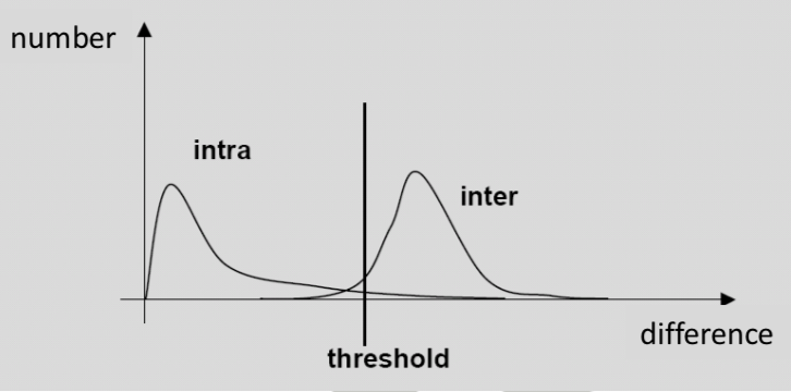
• Choice of threshold is very important
  • Too low: False cuts
  • Too high: Missed cuts
• Threshold depends on video type (application-specific)
• Training:
  • Use a predefined training set
  • Interpret shot as cluster
  • Compute difference of frames inside (intra) a shots
  • Computer difference of frames from different (inter) shots
  • Select point with high intra-cluster similarity and low inter-cluster similarity

Template Matching

• Zhang et al, 1993
• Idea:
  • Pixel-wise comparison of two frames
  • Assume a cut, if change exceeds a threshold
• Change between frames: Difference of pixels \( (x,y) \) of both pixels
• \( D_{cut} = \sum_{x,y} | I(x,y,t) - (x,y,t+1)| \)
• Can only find hard transitions (\( D_{cut}>t \))
• Disadvantage:
  • Noise/change in camera angle have impact
  • Requires predefined threshold

Histogram-based Methods

• Tonomura, 1991
• Assumption:
  • Frames containing identical foreground/background have similar brightness distribution (intensity distribution)
• Histogram columns:
  • Number of pixels with specified value
  • e.g., certain color/brightness
• \( H(j,t) \): Histogram value for brightness \( j \) at time \( t \)
• \( D_{cut}=\sum_j |H(j,t)-H(j,t+1)| \) (L1-norm)
• Personal idea:
  • Use different histogram-metrics
• Advantage:
  • Rotation invariant
  • Histogram changes slightly:
    • Object translation
    • Occlusions by moving objects
    • Slow camera movement
    • Zooming
  • Less error-sensitive (more robust)
• Disadvantage:
  • Requires predefined threshold \( T \)

Twin-Thresholding

• Zhang et al, 1993
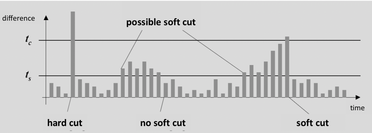
• Problem: Smooth transitions have small change between two frames
• Idea: Use two thresholds
  • One for hard cuts
  • One for soft cuts
• Threshold \( t_c \): Intolerable change (hard transitions)
• Threshold \( t_s \): Detect possible smooth transitions
• Workflow:
  • Mark a frame with difference exceeding \( t_s \) at time \( t \) for a smooth transition as reference frame
  • Then compare frames \( [t+1,t+n] \) against reference frame (\( n \) is collection-dependent)
  • If the difference between reference frame and current frame exceeds \( t_c \), assume a soft cut

Block-based Techniques

• Idris/Panchanathan, 1996
• Goal: Avoid noise/different camera settings
• Idea:
  • Split image into regions/blocks
  • e.g., like in image retrieval
• Method
  • Divide frame into \( r \) blocks
  • Calculate characteristics for each block (e.g., histogram, template matching, …)
  • Compare corresponding sub-frames
• Advantages
  • Detect/ignore effects in only one part of the picture
  • If a high number of the blocks are similar: Same shot

Model-based Procedure

• Idea:
  • Model transitions by mathematical operations
  • e.g., fading, moving image, splitting image
  • Detect characteristic pattern
• Method:
  • Mathematical operation on the brightness histogram
  • Start/end of transitions corresponds to shot boundaries
• Advantage:
  • Recognize transition and their type
• Disadvantage:
  • Collection-dependent
  • Only detect pre-defined transitions (missing those very special ones)
• Example: Fading
  • Fade out: Compress brightness histogram to the left
  • Fade in: Histogram is stretched to the right

Compressed Videos (DETOUR)

• Compressed storage is (obviously) required
• Shot detection on compressed data is a trade-off between efficiency and accuracy
• e.g., use MPEG compression
• MPEG compression
  • Base:
    • Cosine transformation coefficients
    • Motion vectors
  • Idea: Encode changes between frames
  • Frame types:
    • I: Independent code
      • Compressed with DCT
      • Divide image into blocks
      • Each block compressed with DCT
      • DC-frame: Only use first DC-coefficient (average intensity)
      • DC sequence: Sequence of DC-frames
    • P: Predicted
      • With change information from preceding I-frame/P-frame
    • B: Bi-directional
      • Interpolation between P/I- or P/P-frames
      • Computation based on preceding and subsequent frame
• Shot detection:
  • Zhang et al, 1993
  • (Block) Motion vector: Vector for each pixel indicating the change
  • Observation: Frames of the same shot have similar motion vectors

Statistical Models

• Vasconcelos et al., 2000
• Idea:
  • Use perceptional features (e.g., visual structure) instead of low-level features
  • Move away from pixel-based descriptions
  • Decompose video into semantic units and structure (shots, mood, action)
  • Base on film theory (estimate using statistics)
• Film theory:
  • Stylistic elements
    • Montage: Temporal structure of shots (e.g., shot length, cutting)
    • Mis-en-scène: Spatial structure, scenery, lighting, camera position (refers to the image)
  • Emotions: Long passage with text and facial expressions (long shot duration)
• Goal:
  • Build models for stylistic elements Montage and Mis-en-scene
  • Extract semantic features (characterization + classification)
  • Use background information for shot detection
• Example:
  • Shot activity and shot duration correlate (weakly)
  • The shorter the shot, the higher the action

Video Structure

• Categorize by semantic structure
• Film theory leads to more semantics than low-level features
• Assumption:
  • The more structure in a video, the more semantic information
• Classical elements:
  • Montage: Shot duration
  • Mis-en-scene:
    • Shot Activity (explosions, violence)
    • Mood (colors, brightness)
• Disadvantage:
  • Mis-en-scene elements are hard to detect

Shot Duration (Temporal Models)

• Idea:
  • Model shot boundaries as an event
  • Multiple shot boundaries are a sequence of events
• Models:
  • Poisson distribution (Queuing theory)
  • Erlang distribution
  • Weibull distribution
• Training:
  • Use training collection with manual shot boundaries
  • Leads to maximum likelihood estimate

Poisson Distribution

• Idea:
  • Interpret occurrence of shot boundary (cut) by the Queuing theory (arriving people in a queue)
• Queuing theory:
  • Poisson process
  • Number of events in fixed time interval follow Poisson distribution
  • Temporal distance between successive events is exponentially distributed
• Problems:
  1. Many short, few long shots (does not apply to all kinds of videos)
  2. Memorylessness: Probability that in the next \( t \) time units a cut happens is independent of \( t \) (assumption does not hold for movies)

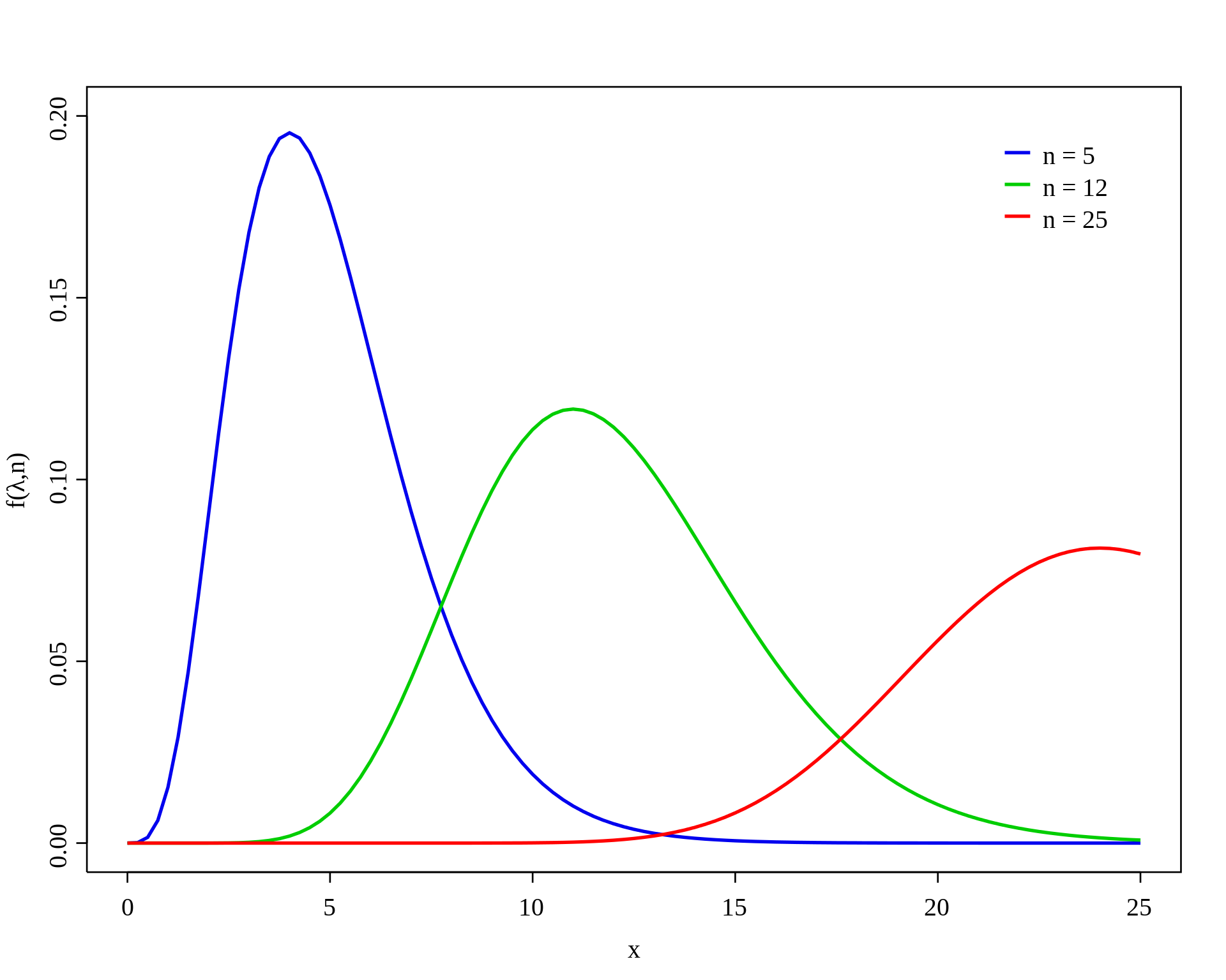
Erlang Distribution

• Assumption: Shot duration is Erlang distributed
• Training:
  • Estimate model parameters from training collection
  • Maximum likelihood estimator
• Formal
  • Event: Semantic event in the shot (NOT the shot boundary)
  • \( \tau \): Time since the last shot (length of the shot)
  • \( r \): Order
    • Required number of events after which as shot boundary occurs
    • e.g., \( r=3 \) means after 3 events occurs a cut: build-up, dialog 1, dialog 2
  • \( \lambda \):
    • Number of events per time unit
    • \( 1/\lambda \): Expected inter-arrival time (time between events)
  • Describes the probability of seeing event \( r \) after time \( \tau \) if we assume \( \lambda \) events per time unit
  • Density function: \( \epsilon_{r,\gamma}(\tau) = \frac{\lambda^r \tau^{r-1} e^{-\lambda \tau}}{(r-1)!} \)
  • Generalization of exponential distribution (\( r=1 \))
  • Expected value:
    • \( \frac{r}{\lambda} \) (time per shot)
    • e.g., \( \frac{3\frac{events}{shot}}{6\frac{events}{min}}=0.5\frac{min}{shot}=2\frac{shot}{min} \)
  • Sum of \( r \) exponential distributions with parameter \( \lambda \) is \( (r, \gamma) \)-Erland distributed
• Likelihood function
  • Single Erlang-distributed random variable:
    • \( \epsilon_{r,\gamma}(\tau) = \frac{\lambda^r \tau^{r-1} e^{-\lambda \tau}}{(r-1)!} \)
  • Log-likelihood function:
    • \( \log\epsilon_{r,\lambda}(\tau)=r\log\lambda+(r-1)\log\tau-\lambda\tau-\log((r-1)!) \)
  • Optimization problem:
    • Discrete variable \( r \)
    • Continuous variable \( \lambda \)
  • Optimize \( r \):
    • Due to film theory \( r \) should be small (a shot does not contain that much happening)
    • Brute-force solution: Test \( r=1,\ldots,10 \) values
  • Optimize \( \lambda \) with given \( r \):
    • \( \lambda* = \frac{Nr}{\sum_i \tau_i} \)
    • \( N \): Independent Erlang-distributed random variables (==Number of shots???==)
• How about the problems?
  • Problem (1): Solved (adaptive for different distributions of shot lengths)
  • Problem (2): Unsolved, still memoryless (use Weibull distribution)

Weibull Distribution

• Not explained in the lecture
• What should the Weibull distribution improve?
  • Generalization of Exponential distribution
  • Has memory (respect previous events)

Shot Activity

• Idea:
  • Use low-level features (e.g., histograms) with film theory
  • Visual similarity within shot boundary frames is higher than for regular frames
• Approach 1: Histograms
  • Difference of color histograms in two consecutive shots
  • \( D(a,b)=\sum_i |a_i-b_i| \) (L1-norm)
  • Goal: Use this information to determine statistical model for shot activity
• Approach 2: Film theory
  • Continuity in editing
  • Shot boundaries should be clearly visible to not confuse the audience
  • Separate frames:
    • Regular frame: \( S=0 \)
    • Shot boundary: \( S=1 \) (frames near shot boundary)
  • Classify each frame into the two classes

Shot Boundary Detection

• Combine Shot Duration and Shot Activity approach
• Use statistical test
  • Given: Two frames \( a \) and \( b \)
  • \( H_0 \): Between the frames is no cut (\( S=0 \))
  • \( H_1 \): Between the frames is a cut (\( S=1 \))

Likelihood Ratio Test

• Choose \( H_1 \):
  • \( D \): Distance between frames \( a \) and \( b \)
  • \( P(D|S=1)>P(D|S=0) \) or
  • \( \log\frac{ \)P(D|S=1)}{\( P(D|S=0)}>0 \)
• Uses no knowledge about shot duration

Bayesian Statistics

• Generalization of Histogram-based thresholding
• Notation:
  • \( \delta \): Duration of each frame (constant)
  • \( S_{t,t+\delta} \): Shot boundary between frame at \( t \) and at \( t+\delta \) (binary)
  • \( D_{t,t+\delta} \): Distance between frame at \( t \) and its successor
  • \( S_t=(S_{0,\delta},S_{\delta,2\delta},\ldots,S_{t,t+\delta}) \)
  • \( D_t=(D_{0,\delta},D_{\delta,2\delta},\ldots,D_{t,t+\delta}) \)
• Hypothesis \( H_1 \) valid:
  • \( P(S_{\tau,\tau+\delta}=0 | S_{\tau},D_{\tau+\delta})>P(S_{\tau,\tau+\delta}=0|S_{\tau}=0,D_{\tau+\delta}) \)
• …
• Erlang model threshold:
  • Estimate the threshold dynamically for time \( \tau \)
  • \( T_\epsilon(\tau)=\frac{\sum_{i=1}^r \epsilon_{i,\lambda}(\tau+\delta)}{\sum_{i=1}^r (\epsilon_{i,\lambda}(\tau)-\epsilon_{i,\lambda}(\tau+\delta))} \)
  • At first, Threshold high (unlikely for cuts)
  • Then, threshold drops
  • Threshold always greater than 0

Experiments

• Vasconcelos/Lippman, 2000