Indexing
Basics
- Problem: Sequential search too inefficient
- Solution:
- Use indexing
- Efficient management of multi-dimensional information
- Data to be indexed:
- Real-valued feature vectors
- Skeletons
- Chain codes/Parsons codes
- Multi-dimensional index:
- Manage multi-dimensional information:
- Pre-structuring of data for search functionality
- Efficient data structures
- Efficient search/comparison algorithms
- Use list semantics
- Ranking of results by the degree of how well they satisfy the query
- Manage multi-dimensional information:
Requirements
- Correctness of indexing algorithm
- Completeness of indexing algorithm
- Support for non-real-valued vectors (i.e., non metric)
- Support multiple distance functions
- Support different query types
- Exact search / point query
- k-Nearest-neighbor search
- Scalability (w.r.t. number of dimensions)
- Efficient update complexity
- Efficient sub-linear search complexity
- Low memory usage
Tree Structures
- Relational databases:
- B-Tree (one-dimensional)
- Exact search and logarithmic cost
- Node size: One disk block
- Multimedia database:
- Multi-dimensional tree
- Idea:
- Describe set of points by using geometric regions
- Use these clusters for the search
- Hierarchical structure
- Classification of tree structures:
- Cluster construction (fragment entire space vs. group data)
- Cluster overlap (overlap vs. disjoint)
- Balance (unbalanced tree vs. balanced)
- Object storage (object only in the leaves vs. objects in inner nodes + leaves)
- Geometry (hyper-sphere, hyper-cube, …)
R-Trees
Basics
- Guttman, 1984
- Multi-dimensional extension of the B-Tree
- Maximal dimensions:
- R-Tree: 10
- R+-Tree/R*-Tree/X-Tree: up to 20
- Dynamic index structure (support changes)
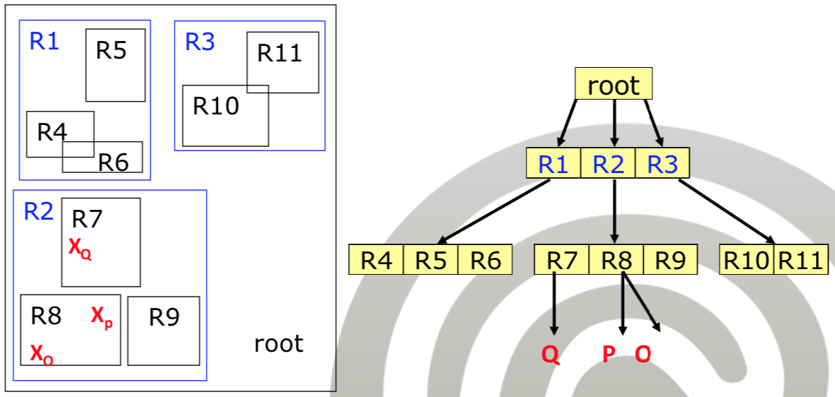
- Data structure:
- Data pages: Leaf nodes (store data objects and clustering data)
- Directory pages: Inner nodes (store directory entries, used for navigation)
- Structure uses Minimum Bounding Rectangles
Classification
- Cluster construction: Local grouping
- Cluster overlap: Overlapping
- Balance: Balanced
- Object storage: Leaves only
- Geometry: MBRs
Structure
- Pre-defined parameters:
- \( M \), \( m\leq M/2 \)
- \( M \) corresponds to the size of a disk block
- Root node:
- At least two children
- Internal node:
- Multiple entries \( (I, \text{child-pointer}) \)
- \( I \): Smallest rectangle containing all children
- Has between \( m \) and \( M \) children
- Leaf node:
- Multiple index entries \( (I, \text{tuple-ID}) \)
- \( I \): Bounding rectangle/coordinates of the data object tuple-ID
- All leaves are on the same height
- All leaves have between \( m \) and \( M \) records
Block Access Cost
- Important for good cost / efficient search:
- Minimal overlap
- Minimal dead space
Operations
- Search
- Insert
- Update
- Delete
- Split
Search
- Query: Rectangle \( Q \)
- Search recursively from root to leaves
- Select one path to child (arbitrary)
- Search in child
- If object not found, traverse next path
- Performance: No guarantee
- Worst case: Traverse all paths (for overlapping MBRs)
- Use pruning of irrelevant regions
- Searching internal nodes:
- Check each \( I \) from \( (I, C) \) for intersection with \( Q \)
- For all intersecting children, continue with them
- Searching leaf nodes:
- Check entries whether they are in \( Q \)
- Add objects to result set
Insert
- Goal: Choose best leaf page
- Use leaf requiring the smallest volume growth
- Heuristic:
- Always, prefer smallest volume growth (leads to less dead space)
- Steps:
- Find a leaf
- Case A) Data point falls directly into an MBR
- Case B) Data point requires the enlargement of another MBR
- Enlargement: Select the MBR with the smallest volume growth and ignore overlaps
- Splitting
- Required if the leaf contains \( M \) objects
- Also called Overflow Problem
- After splitting, adapt the parent node (the split may propagate to the root)
- Goal:
- Keep the tree balanced
- Avoid traversing two subtrees
- Resulting MBR volumes should be as small as possible
- Approaches
- Quadratic Splitting
- Linear Splitting
- Find a leaf
Quadratic Splitting
- Starting points: Use the points with the largest MBR (these points are not in the MBR)
- For each object
- Compute the volume increase to MBR 1 and MBR 2
- Select the object with the maximal difference of volume increases (smallest volume increase to either MBR 1 or MBR 2)
- Stopping criteria:
- At least one MBR contains \( M-m+1 \) objects
- Then, assign the remaining objects to the other MBR
Linear Splitting
- Also called Greene’s Split
- Simplification of the quadratic method
- For each axis
- Compute the distance \( \text{diff}_{\text{dim}} \)
- Select the rectangle with the highest minimum coordinates
- Select the rectangle with the smallest maximum coordinates
- Subtract values
- Note: \( \text{diff}_{\text{dim}} \) corresponds to the dead space in this dimension
- Divide it by the maximum distance on this axis (i.e., the difference between the smallest minimum and highest maximum coordinate)
- e.g., \( d_x = \text{diff}_x / \max_x \)
- Compute the distance \( \text{diff}_{\text{dim}} \)
- Starting point:
- Rectangles with the highest normalized distance
- Normalized dead space
- For each object:
- Sort by minimum rectangle values on the selected axis
- Add to the nearest MBR on the selected axis
Delete
- Search corresponding leaf node
- Delete the object
- IF number of objects less than \( m \)
- Condense the tree
- Delete all objects of the node
- Re-insert them
- IF the root has only one child
- The child becomes the new root
Update
- If the corresponding MBR changes, delete the entry and re-insert it
R+-Trees
- Problem with R-Tree: Allow for overlaps
- Sellis et al., 1987
- Idea:
- Prohibit overlapping MBRs
- No minimum number of children
- Result:
- Identical leads may occur more than once
- Improved search efficiency
- Similar scalability (10 dimensions)
- Insert Operation:
- Object can be inserted into multiple leaves
- Splitting propagates up- and downwards (no overlap allowed)
- Advantage:
- R+-Tree saves 50 % of access time
- Disadvantage:
- Objects stored multiple times
- Low filling of nodes
- Degeneration for increasing number of changes (no balancing)
M-Trees
- Ciaccia et al., 1997
- Metric Trees
- 15-20 dimensions
- Idea: Use arbitrary (non-euclidean) metrics
- e.g., editing distance
- Underlying concept: Triangle equality for pruning
- Only use distance information (no geometry)
- Metric space
- \( M=(U,d) \)
- \( U \): Universe
- \( d:U\times U\rightarrow \mathbb{R} \): Metric
- No clear geometry (instead of Euclidean space)
- Classification:
- Clustering: Local grouping
- Cluster overlap: Overlap
- Balance: Balanced
- Object store: Leaves only
- Geometry: Hyper-sphere (ellipse)
Triangle Equality
- \( \forall x,y,z: d(x,z)\leq d(x,y)+d(y,z) \)
- All distances of points are pre-computed (symmetric matrix)
- Query \( Q \)
- Goal: Find closest point to \( Q \)
- Requires distance to some point \( p \): \( d(Q, p \))
- Estimate distance to other points
- Compute lower limit for the distances
- \( d(Q, p) \leq d(Q, q) + d(p, q) \)
- \( d(Q, q)\geq d(Q, p)-d(p,q) \)
Structure
- Node size corresponds to disk block size
- Upper and lower bounds (like in the R-Tree)
- Internal nodes
- Routing object \( v_N \)
- Covering radius \( r_N \)
- Distance to parent node \( v_P \)
- Leaf node
- Indexed objects
- Distance to parent node
Formalization
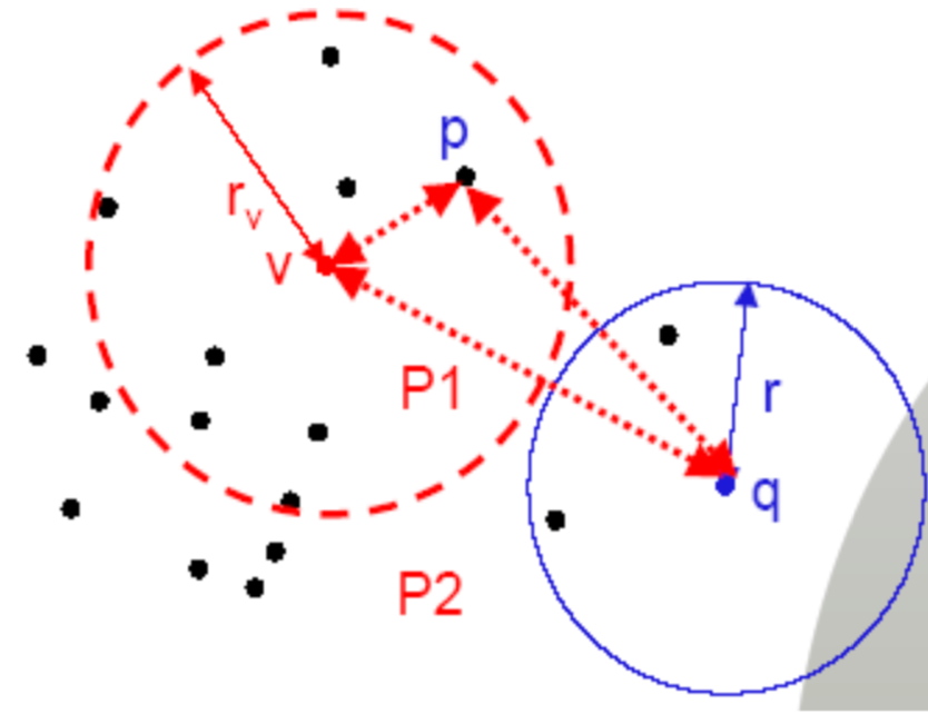
- Partition data objects in \( \epsilon \) environment
- Radius \( r_v \)
- \( P_1=\{p\mid d(p,v)\leq r_v\} \)
- \( P_2=\{p\mid d(p,v)> r_v\} \)
- \( |P_1|\approx |P_2|\approx \frac{|P|}{2} \)
- Region \( Reg(N) \)
- Node \( N \)
- Routing object \( v_N \) (center)
- Radius of the area \( r_N \) (covering radius)
- \( Reg(N)=\{p\mid p\in U, d(p, v_N)\leq r_N\} \)
- All points \( p \) have guaranteed distance of at most \( r_N \) to \( v_N \)
Fast Pruning
- Query \( q \):
- Query has a radius \( r_q \)
- What is considered similar
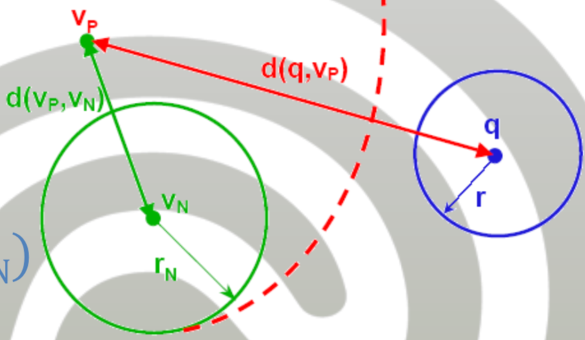
- Prune node \( v_N \):
- \( d(q, v_N) > r_q + r_N \)
- Fast Pruning:
- Node of interest: \( v_N \)
- Parent node: \( v_P \)
- \( d(q, v_P)\leq d(v_P,v_N)+d(v_N, q) \)
- \( \iff |d(q,v_P)-d(v_P),v_N)| \leq d(q, v_N) \)
- Pruning criterion:
- \( r_N+r_q<|d(q,v_P)-d(v_P,v_N)| \)
Search Operation
- Recursively start from root
- Steps:
- Compute distance to root: \( d(q, v_{root}) \)
- Perform fast pruning for every child node of the root
- Search the nodes where the pruning criterion does not hold
Insert Operation
- Goal: Smallest expansion of the radius
- Overflow: Perform split
- Choose two new routing objects
- Heuristic: Minimize difference between the two new radiuses (i.e., similar size of spheres)
- Balanced Split: Add objects iteratively to their neighbors
Curse of Dimensionality
- Richard Bell
- Central question:
- Why does the efficiency of multi-dimensional index structures fail after 15-20 dimensions?
- Can we create an efficient high-dimensional tree?
- Problem:
- Index trees fail after 15-20 dimensions of uniformly distributed data
- Costs are higher than a linear scan
- Volume of space grows exponentially with the number of dimensions
Basic Geometry
- Uniform, random sampling within a cube of unit length
- Two cubes:
- One cube with edge length \( 1 \)
- Another cube with edge length \( (1-2\epsilon) \)
- The higher the dimensions, the volume of the inner cube becomes very low
- Result: Huge number of samplings so that one is inside the inner cube
- Distances:
- How many points have exactly distance \( s \) from the center?
- The higher the dimensions, the lower the variance
- The higher the dimensions, the farther apart are the points
- Result: Almost all points have same distance to the query
- Result:
- Sequential search is often faster
- Real-world data may have intrinsic lower dimensionality (e.g., price and speed for vehicles)
Vector Approximation Files
- Weber et al. 1998
- Goal: Speed up sequential search
- Idea:
- Partition the space into hyper-cubes
- Identify each partition with a bit-string
- Identify each object with the bit-string of its partition
- Approximate the vector-representation
- Formally
- \( d \) dimensions
- Represent dimension \( i \) with \( b_i \) bits
- Split dimension \( i \) in \( 2^{b_i} \) intervals
- Represent a point approximately by \( b = b_1+\ldots+b_d \) bits
- e.g., \( (0.1, 0.6) \) by \( 0010 \)
- Advantage:
- For a large enough \( b \), there are more partitions than data points, which reduces the number of collisions.
- Bit-wise operations are faster
- Query processing:
- Query with radius yields a set of partitions (thus, bit-strings)
- Sequential scan over all partitions
- Intersect partition with search region
- Check all contained points using the exact coordinates
Dimensionality Reduction
- Idea:
- Reduce dimensions to the ones containing essential information
- Combine strongly correlated dimensions
- Methods:
- Principal component analysis
- Latent Semantic Indexing
- Problem: Frequent data change
- Data change could affect the results of the transformations
- Solution: Use representative portion of the data for all objects
Principal Component Analysis
- Karhunen-Loeve transform
- Idea:
- Detect linear dependencies between features (sign of redundancy)
- Rotate and shift the axis resulting in no linear dependency between the new axis
- Remove axis with low variance (keep the error minimal)
- Center the coordinate system
- Center around the mean
- \( X=(X_1,\ldots,X_d) \)
- \( \hat{X}=(\hat{X_1},\ldots,\hat{X_d}) \)
- \( \hat{X_i}=(X_i-E(X_i)) \)
- Covariance matrix:
- Covariance: \( cov(X,Y)=E(X\cdot Y) \)
- Covariance matrix contains pair-wise covariances
- Dimensions containing non-zero covariance carry redundant information
- Diagonalize the covariance matrix:
- Eigenvalue decomposition
- \( A=Q\cdot D\cdot Q^{-1} \)
- \( Q \): Orthogonal \( Q^T=Q^{-1} \) (rotation)
- \( D \): Diagonal matrix containing the eigenvalues (scaling)
- Multiplication of the data with \( Q \) maps it into low-dimensional space
- Remove dimensions with small eigenvalues (small information)
Latent Semantic Indexing
- Idea:
- Decompose feature matrix \( F \) (feature vectors as columns)
- Represent vectors by its latent semantics (the axis)
- Use case:
- Synonyms in information retrieval
- Differentiate between the concepts of ambiguous terms
- \( F = U\cdot D\cdot V^T \)
- \( U \):
- Left-singular vectors (orthonormal)
- Feature dimensions (to latent space)
- \( D \): Singular matrix
- Contains singular values
- Higher singular value -> higher meaning
- Only keep \( 1\leq k\leq d \) dimensions
- \( V_T \):
- Right-singular vector (orthonormal)
- Feature vectors (to latent space)
- \( U \):
GEMINI Indexing
- GEneric Multimedia Object INdexIng
- Faloutsos, 1996
- Idea:
- Use a simple distance function instead of a complex one to compute a lower bound
- Use for pruning (e.g., average color)
- Formally
- Complex distance \( d_C(a,b) \)
- Set of objets \( O \)
- Choose transformation function \( f:O\rightarrow K \)
- Choose simple distance function \( \delta: K\rightarrow \mathbb{R} \)
- Lower Bounding Property: \( \forall a,b\in O: \delta(f(a), f(b))\leq d(a, b) \)
- Algorithm:
- Preparation:
- Transform database objects using \( f \)
- Pruning:
- Region query \( (q, r) \)
- Exclude objects \( a \) with \( \delta(a, q)>r \)
- Processing:
- Compute \( d(b,q) \) for all remaining objects \( b \)
- Exclude objects \( b \) with \( d(b,q)>r \)
- Preparation:
- Nearest-neighbor query \( q \)
- Nearest neighbor for \( \delta \) is not always the nearest neighbor according to \( d \)
- Compute nearest neighbor \( a \) according to \( \delta \)
- Compute \( d(a, q) \)
- Perform a range query \( (q, d(a, q)) \)
- Perform nearest neighbor query on the results of the range query
Fast Map
- Faloutsos and Lin, 1995
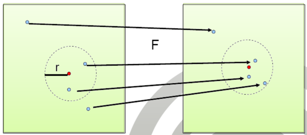
- Goal: Simplify complicated distance functions
- Idea:
- Represent database objects as points in \( \mathbb{R}^k \) for some distance function \( d \)
- \( k \) is predefined
- Higher \( k \): More accuracy
- Lower \( k \): More efficiency
- Requirements:
- Efficient mapping (linear complexity)
- Good distance approximation
- Efficient mapping of new objects
- Method:
- Assume, objects are already in Euclidean space (without knowing their coordinates)
- Find \( k \) orthogonal axis based on the other points
- Project points on these axis
- Cosine: \( d(A,X)=\frac{d(A,C)^2+ d(A,B)^2- d(B,C)^2}{2\cdot d(A,B)} \)
- Example:
- Triangle with points A, B and C
- Project C on the axis of A and B: Point X
- Represent C in the term of \( d(A, X) \)
- Algorithm:
- Project objects on a hyperplane (normal vector is the new axis)
- Compute coordinates using two pivot elements
- Repeat \( k \) times
- Pivot elements:
- Choose objects being farthest apart (least loss of accuracy)
- Quadratic cost vs. linear cost