Models
Boolean Retrieval
- Document: Set of words
- Query:
- Propositional formula with (AND, OR, NOT)
- Processing:
- Convert query to disjunctive normal form
- Use inverted index
- Intersect posting lists (sorted, \( O(N) \))
- Optimization: Start with smallest intermediate result / sort terms by increasing document frequency
- Advantages
- Easy to understand
- Theoretically powerful (every possible subset can be retrieved)
- Disadvantages
- No ranking
- No similarity queries
- Low recall (e.g., synonyms)
Fuzzy retrieval model
- Motivation
- Index terms are not equally important/characteristic (e.g., synonyms, multiple incidences)
- Assign weight to terms
- Idea
- Based on boolean retrieval
- Use fuzzy result sets (continuous degree of membership)
- Central questions
- How to answer queries?
- How to get the membership degrees?
- Advantages
- Support for non-binary assignment of index terms
- Support for synonyms/related terms
- Ranking
- Disadvantages
- Difficult computation
- Un-intuitive querying
Representation
- Query:
- Propositional formula (as in boolean retrieval)
- Alternative operators: t-Norm, t-Conorm
- Document:
- Bag-of-words (set-of-words makes more sense)
- Each term has a membership degree
- Terms in the document have degree \( \mu(t) = 1 \)
- Additional terms have degree \( \mu(t) \leq 1 \)
- Processing:
- Use Zadeh operators
- Problem: Strange behavior
a={x/0.4, y/0.4} b={x/0.3, y/1.0} q=x AND y r={x/0.4, y/0.3}
Membership degree
- Ogawa et al., 1991
- Use co-occurrence of terms
- Jaccard index \( J(t_1, t_2) \)
- Also called term-term correlation coefficient
- Problem: Jaccard index does not mention the documents not containing any of the two terms
- \( J(t_1, t_2) = \frac{df(t_1\land t_2)}{df(t_1 \oplus t_2)} \)
- Computation:
- \( W(d, t) = 1- \Pi_{u\in d} (1-J(t,u)) \)
- Idea:
- \( 1-J(t,u) \) measures dissimilarity of \( t \) and \( u \)
- The more often a term co-occurs with all terms of a document, the more similar is the term to the document
Coordination level matching
- Luhn
- Idea:
- User sketches document
- Document with an overlap of terms of size \( n \) is more relevant than a document with overlap of size \( n-1 \)
- Query:
- Bag-of-words (virtual document)
- Document:
- Bag-of-words
- Processing:
- Compute coordination level (size of overlap)
- Ranking with the coordination level
- Alternative: Scalar product of binary term incidence vectors
- Advantages
- Easy comparison
- Disadvantage
- No support for synonyms
Vector space model
- Salton, 1975
- Idea:
- Represent documents as points in space (as in libraries)
- Use proximity as similarity measure
- Document:
- \( d\in \mathbb{R}^{n} \)
- Index term spans own dimension
- Term weighting approaches
- Binary incidence (set-of-words)
- Fuzzy membership degree
- Term-frequency (bag-of-words)
- Term-frequency and term discrimination
- Processing:
- Convert query to binary-incidence-vector
- Scan postings lists for each query term
- Sum up scores for each document
- e.g., term frequency, TF-IDF
- Similarity measure: Scalar product (ranking)
- Important questions
- Which similarity measure to use?
- How to assign weights to terms?
- Applications
- Scoring/retrieving documents
- Document classification
- Document clustering
- Advantages
- Simple/clear
- Intuitive querying
- Customizable (similarity, normalization, term weighting)
- High retrieval quality
- Relevance feedback (e.g., Rocchio)
- Disadvantages
- High dimensionality (curse of dimensionality)
- Word order is lost
- Implicit assumptions
- Cluster hypothesis
- Independence/orthogonality assumption
Similarity
- Measure \( s:X\times X\rightarrow [0,1] \)
- \( s(x,y) = 1 \): Maximal similar
- \( s(x,y)=0 \): Maximal dissimilar
- Example:
- Cosine similarity
- \( s(x,y) = cos(\measuredangle(x,y)) = \frac{x*y}{||x||*||y||} \)
- Choice of similarity measure
- Depends on application
- Options:
- Cosine similarity
- Euclidean distance
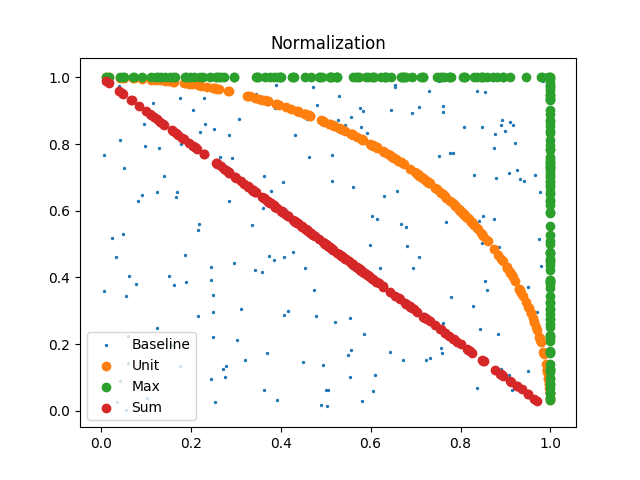
Normalization
- Why?
- Euclidean distance depends on vector length
- Cosine similarity does not depend on length
- Approaches
- Divide by length / normalize to unit length
- Divide by max. coordinate
- Divide by sum of coordinates
- Advantage Divide by length
- Vector norm equals \( 1 \)
- Computation of cosine similarity is cheaper (unit length)
- Rank created by euclidean distance is the same as for cosine similarity
- Problem: Longer documents are more in-depth
- Solutions:
- Compute result normally and boost long documents
- Measure effect of document length on relevance and adjust ranking
Term weighting
- Term frequency \( tf(d, t) \)
- Luhn, 1961
- Repetition of words is an indication of emphasis
- Discrimination \( disc(t) \)
- Not every term equally important (e.g., stop words)
- Approaches
- TF-IDF
- Document structure
- Idea:
- High term frequency -> High term weight
- High discriminative power -> High term weight
- \( w(t) \propto tf(d,t) * disc(t) \)
TF-IDF
- Spärck Jones, 1972
- Idea:
- Term specificity as term discrimination
- The more specific a term is, the larger its discriminative power is
- Normalize with respect to collection size
- Use inverse document frequency \( df(t)^{-1} \)
- Relationship specificity and inverse document frequency is logarithmic
- Formula:
- \( tf(d,t) * \log(\frac{N + 0.5}{df(t) + 0.5}) \)
Document structure
- Idea:
- Use structure of document collection
- Removing a highly discriminative term leads to large change in average document similarity
- Remove a non-discriminative terms leads to small change in average document similarity
- Formalization:
- \( s \): Similarity measure between documents
- \( s_{avg} \)
- Average similarity across all documents
- \( s_{avg} =\frac{1}{N^2} \sum_ {d,e\in C}s(d,e) \)
- \( s_{avg,t} \)
- Average similarity across all documents
- Remove dimension corresponding to term \( t \)
- \( disc(t) = s_{avg} - s_{avg,t} \)
- Problem: Expensive computation
- Solution: Heuristics (compute average document, leads to linear runtime)
Comparison to boolean and fuzzy retrieval
- Vector space model has better average precision using fixed recall
Probabilistic retrieval
- Base of probabilistic IR: Probabilistic ranking principle
- Models
- Probabilistic indexing
- Binary Independence model (+ extensions)
- Poisson model
- Belief networks
- Advantages
- Good in experiments
- Intuitive measure
- Well-defined mathematical foundations
- Explicit assumptions
- Disadvantages
- Parameter estimation difficult
- Doubtful assumptions (e.g., independence)
- Less flexible than vector space model
- Complicated
Probabilistic Ranking Principle
- Robertson, 1977
- Principle:
- If result list is ordered decreasingly by probability of usefulness, the effectiveness of the system is the best that is obtainable
- Important: Probability of usefulness is estimated as accurately as possible on the given data
- Usefulness: Hard to define
- Relevant documents:
- \( R_q = \{d\in C\mid \text{d relevant w.r.t q}\} \)
- Task:
- Input: Query \( q \), document \( d \)
- Output: \( P(d\in R_q) \) (Bayesian interpretation)
- \( R_q \) is unknown, estimate using other probabilities
Probabilistic Indexing model
- Maron/Kuhns, 1960
- Idea: Improve search on manually indexed collections
- Notion:
- \( k \) index terms
- Document \( d\in [0,1]^k \) (weighted)
- Query \( q\in \{0,1\}^k \) (binary)
- Task: Estimate \( P(d\in R_q) \)
- Random variable \( Q \)
- Over all possible queries
- Distribution given by query logs
- Random set of documents \( R_Q \)
- Formula: \( P(d\in R_q) = c(q) * P(d\in R_Q) * \Pi_{i\in \{i,...,k\}, q_i=0} (1-d_i) * \Pi_{i\in \{i,...,k\}, q_i=1} d_i \)
- Important assumptions
- Independence
- Maron’s and Kuhn’s argument
Estimation
Overview
- Assume \( P(d\in R_q) = P(d\in R_Q\mid Q=q) \)
- Apply Bayes’ theorem
- Replace \( P(Q=q) \) with constant \( c(q) \)
- \( P(Q=q) \) equal for all documents
- Estimate \( P(d\in R_Q) \) with relevance feedback
- Model for general relevance
- Relative frequency of positive ratings
- Proportional to \( P(d\in R_q) \)
- Assume independence of query terms
- Not reasonable (co-occurrence, synonyms)
- Split product and use complementary events
- Maron/Kuhns’ argument
- Use term weight for probability \( P(Q_i=1\mid d\in R_Q) \)
- Assigned by human indexer
- Indexer knows relevance to topics
- Optional: Ignore non-occurrence
- Most users leave out query terms
Estimation of \( P(Q=q\mid d\in R_Q) \)
- Independence of query terms
- \( = \Pi_{i=1}^k P(Q_i=q_i\mid d\in R_Q) \)
- Split product
- \( = \Pi_{i\in \{i,...,k\}, q_i=0} P(Q_i=0\mid d\in R_Q) * \Pi_{i\in \{i,...,k\}, q_i=1} P(Q_i=1\mid d\in R_Q) \)
- Complementary events
- \( = \Pi_{i\in \{i,...,k\}, q_i=0} (1-P(Q_i=1\mid d\in R_Q)) * \Pi_{i\in \{i,...,k\}, q_i=1} P(Q_i=1\mid d\in R_Q) \)
- Maron and Kuhns’ argument
- \( = \Pi_{i\in \{i,...,k\}, q_i=0} (1-d_i) * \Pi_{i\in \{i,...,k\}, q_i=1} d_i \)
Binary independence model
- Rijsbergen, 1977
- Notion:
- \( k \) index terms
- Document \( d\in \{0,1\}^k \) (binary)
- Query \( q\in \{0,1\}^k \) (binary)
- Random variable \( D \)
- Uniformly distributed over all documents in collection
- \( P(d\in R_q) = P(D\in R_q\mid D=d) \)
- Only look at events where \( D \) equals \( d \)
- Ranking: \( O(d\in R_q) \approx \Pi_{i\in \{i,...,k\}, d_i=1, q_i=1} (\frac{P(D_i=1\mid D\in R_q)}{1-P(D_i)=1\mid D\in R_q)}*\frac{N}{df(t_i)}) \)
- Important assumptions
- Linked dependence (weights assigned by indexer)
- Equal term distribution for non-query-terms for relevant and non-relevant documents
- Number of non-relevant documents is approximately \( N \)
Estimation
- Use odds for ranking (strong monotony)
- Apply Bayes’ Theorem
- Replace \( P(D\in R_q) \) with constant \( c(q) \)
- Reduce the fraction by \( P(D=d) \) (fraction is known but numerically useless)
- Intermediate: \( O(d\in R_q)=c(q)*\frac{P(D=d\mid D\in R_q)}{P(D=d\mid D\notin R_q)} \)
- Assume linked dependence
- \( \frac{P(D=d\mid D\in R_q)}{P(D=d\mid D\notin R_q)} = \Pi_{i=1}^k \frac{P(D_i=d_i\mid D\in R_q)}{P(D_i=d_i\mid D\notin R_q)} \)
- Not reasonable (e.g., synonyms)
- Split up by \( d \)
- Use complementary probability
- \( P(D_i=0\mid D\in R_q) = 1-P(D_i=1\mid D\in R_q) \)
- Split up by \( q \)
- Assume identical term distributions for non-query terms for relevant and non-relevant documents
- User queries relevant terms
- \( q_i=0 \Rightarrow P(D_i=1\mid D\in R_q) = P(D_i=1\mid D\notin R_q) \)
- Reduce fraction
- Multiply by 1
- \( 1=\Pi_{i\in\{1,...,k\}, d_i=1,q_i=1} \frac{1-P(D_i=1\mid D\in R_q)}{1-P(D_i=1\mid D\notin R_q)} * \frac{1-P(D_i=1\mid D\notin R_q)}{1-P(D_i=1\mid D\in R_q)} \)
- Replace document-independent block by constant (merge \( d_i=0 \) with \( d_i=1 \)
- Regroup
- Assume \( P(D_i=1\mid D\notin R_q)\approx P(D_i=1) \)
- Number of non-relevant documents is approximately \( N \)
- \( P(D_i=1) \approx \frac{df(t_i)}{N} \)
- Assume \( N >> df(t_i) \)
- Estimate \( \frac{1-P(D_i=1\mid D\notin R_q)}{P(D_i=1\mid D\notin R_q)} \approx \frac{N}{df(t_i)} \)
- Estimate \( P(D_i=1\mid D\in R_q) \)
- User feedback/initial query results
- Croft/Harper (1979): Constant 0.9
- Greiff (1998): \( \frac{df(t_i)}{N} \)
Language models
Motivation
- Observation:
- Different styles of writing
- Documents use different vocabulary
- Idea:
- Represent document by language model (generative model)
- Each topic/document has a specific language
- Find document which language model generates the query
- Approaches
- Formal grammars
- Statistical language models
- Probabilistic context-free grammars (not considered)
Formal grammars
- Describe correct syntax
- Problem: Does not capture style
- Writing style depends on statistical properties
- Solution: Add probability distribution over terms
Statistical language models
- Idea:
- Ignore syntax/grammar
- Focus on statistical regularities
- Use generative model
- Central questions
- Which language model to use for documents?
- How to estimate the language model for each document?
- Applications
- Document generation
- Document recognition
- Use generation probabilities
- e.g. OCR, speech recognition
- Advantages
- Clear statistical foundation
- No ad-hoc weighting
- Better than vector space model
- Disadvantages
- Independence assumption (unigram model)
- Relevance feedback difficult
- No explicit notion of relevance
Assumptions
- Each document has (unknown) statistical document model
- Document is random sample
- Query is random sample of language model of the user’s information need
Definition
- A statistical language model is a probability distribution over sequence of words
- Document \( (w_1,...,w_n) \) gets probability of generation \( P(w_1,...,w_n) \)
- Document length \( n \)
Query processing
- Estimate language model for each document
- For each model, compute the probability of generation for the query
- Rank by probability \( P(q\mid M_d) \)
Models
- Unigram model
- Statistical independence assumed / no context
- \( P(w_1,...,w_n) = P(w_1)*...*P(w_n) \)
- Bigram model
- Context: Previous term
- \( P(w_1,...,w_n) = P(w_1)*P(w_2|w_1)*...*P(w_n|w_{n-1}) \)
- Trigram model
- \( P(w_1,...,w_n) = P(w_1)*P(w_2|w_1)*P(w_3|w_1,w_2)...*P(w_n|w_{n-2},w_{n-1}) \)
Model selection
- Use unigram model
- Reduced computational complexity
- Reduced model complexity (bias-variance tradeoff)
- Losses from data sparseness (short documents, not enough information for conditional probability)
- Sufficient for IR to judge topic
Probability estimation
Maximum likelihood estimator
- \( P(w_i) = \frac{tf(d, w_i)}{n} \)
- Problem: Document often too small
- Missing terms have zero probability
- Occurring terms are overestimated (occurrence by chance)
- Solution: Smoothing
- Add probability to missing terms
- Move probability to collection mean
Smoothing
- Additive smoothing / Laplace smoothing
- Add \( \alpha \) to term frequency (used in TF-IDF)
- Renormalize (to reach sum of one)
- Linear smoothing
- Blend between overall probability of term occurrence and document-specific probability (useful for homogeneous collections)
- \( P(w_i)= \lambda \frac{tf(d, w_i)}{n} + (1-\lambda)\frac{cf(w_i)}{N} \)
- \( \lambda \in [0,1] \): Weighting parameter
- Ponte and Croft (1998)
- Use collection data to stabilize model
- For absent term: Estimate probability over collection (MLE for collection)
- For present term: Smooth MLE with average MLE
Latent Semantic Indexing
- Naive approach: Manual indexing of topics (better: automatically)
- Called Latent Semantic Analysis
- Advantages
- Good quality
- Use synonyms and polysemy
- Mathematical foundation
- Enhancing data quality (removing noise)
- Document can be folded into the latent space
- Disadvantages
- No negations
- No boolean conditions
- Computationally expensive
- Based on Reduced Singular Value Decomposition
- \( S=U\Sigma V^T \)
- \( U \) contains term coordinates
- \( V^T \) contains document coordinates
Motivation
- Vector space doesn’t represent Synonymy and Polysemy
- Synonymy: Two words have the same meaning (document with “car” and “automobile” would be underestimated)
- Polysemy: One word has multiple meanings (document with “charge” would be overestimated)
- Reason: Words assumed to be independent (each word one dimension)
- Idea
- Change basis to dimensions with variance
- Use \( k \) latent topics instead of terms
- Called Semantic space
- Exploit underlying structure of terms and documents
- Connect terms, documents and query with these topics
- Group related terms together (reorder columns/rows) to find components
- Use interrelationships of terms using transitive co-occurrence (car/driver and auto/driver but not car/auto)
- Change basis to dimensions with variance
Low-rank approximation
- Use low rank approximation of the SVD of term-document matrix
- Effects
- Terms with high co-occurrences move together in low dimensional space (synonyms, Why?)
- Terms with several meanings are assigned to several topics (polysemes)
- Noise is removed for correct \( k \)
- \( S \) can be a term-document-matrix with binary incidence
- \( SS^T \) is term-term co-occurrence matrix
- Symmetric matrix
- Cell \( s_{i,j} \) indicates in how many documents terms \( t_i \) and \( t_j \) co-occur (\( S \) binary incidence matrix)
- Reorder high-valued components to get topics
Optimization
- Move singular values into left- and right singular vectors
- \( U_k' = U_k * \sqrt{\Sigma_k} \)
- \( (V_k^T)' = \sqrt{\Sigma_k} * V_k^T \)
- Row of \( U_k * \sqrt{\Sigma_k} \) contains term coordinates
- Column of \( \sqrt{\Sigma_k} * V_k^T \) contains document coordinates
Querying
- Like in vector space
- Map query \( q \) to latent query \( q' \)
- Compare to documents (in latent space)
- Query
- \( q = (U_k^T)' q' \)
- \( q' = \Sigma_k^{-1} * (U_k^T)' * q \)
- Documents in latent space
- \( \sqrt{\Sigma_k} * V^T_k \)
Computation
- Expensive/difficult (even for medium term-document matrix)
- Parameter \( k \) hard to estimate
- Depends on collection
- Too low: Some topics not covered
- Too high: Performance degradation, noisy data
- Optimal: Guess number of topics
Evaluation
- Dumais/Landauer (1993, 1995)
- TREC corpus
- SVD computing using Lanczos algorithm
- Results
- Reducing \( k \) improves recall
- \( k \) in the low hundreds increases precision for some queries (remove noise)
- Netflix Prize